Python I

Getting Started with Python

Training Session Date

Tue. Oct 13, 2026 – 6:00 pm

This training session introduces the fundamental concepts, common data structures, and packages necessary to get started with using Python for data analysis. It will cover the following:

Python Fundamentals
Data Types and Operators
Control Flow
Intro to Pandas library
Appendix

Download the Code and Dataset

You can download this notebook and open it in any Jupyter-compatible IDE, such as JupyterLab, VS Code, Positron, RStudio, or Spyder.

Ensure that you are running at least Python 3.11 and that the necessary package dependencies (pandas, numpy, requests, and others noted throughout the notebook) are installed.

PythonI_Training.ipynb

Python_Data.csv

Using Google Colab

This workbook can also be run in the cloud using Google Colab, with no local setup required. Google Colaboratory (Colab in short) is built on top of Jupyter notebooks and has added functionalities that are found in more conventional IDEs like PyCharm, RStudio, Spyder, etc.

Colab is entirely cloud-based and the free-tier even allows for some free GPU and TPU processing capabilities. Additionally, it can connect with your Google Drive storage for accessing and storing data.

Introduction

Jupyter Notebooks

Earlier called the IPython notebook (hence the .ipynb extension), Jupyter notebooks are an open-source web application that allows you to create and share documents that contain live code, equations, visualizations, and narrative text. They are widely used for data cleaning and transformation, numerical simulation, statistical modeling, data visualization, machine learning, etc.

Jupyter notebooks are a great way to learn and practice Python, as they allow you to run code in small chunks (called cells) and see the output immediately. You can edit a Jupyter notebook in your browser or in a program (called an IDE, short for Integrated Development Environment) like VS Code or RStudio. You can also run Jupyter notebooks in the cloud using Google Colab.

If you want to install Python and Jupyter notebooks on your local machine, we recommend you use an “environment manager” like Anaconda, venv, uv, or pyenv, which can help prevent package conflicts as you install more Python libraries in the future. If you don’t have Python installed on your machine, you can follow this guide to install Anaconda.

Common shortcuts

Jupyter Notebook cells have 2 modes, ‘Command’ and ‘Edit’.

To switch from command to edit mode press Enter. To switch from edit to command mode press Esc.

Execute cell: Ctrl+Enter Execute cell and move to next cell: Shift+Enter (This will add a new cell below if none exists) Execute cell and add new cell below: Alt+Enter

In command mode: - insert cell above: a - insert cell below: b - change cell type to Markdown: m (Ctrl+mm in Colab) - change cell type to code: y (Ctrl+my in Colab) - delete cell: dd (Ctrl+md in Colab)

Setup

Google Colab Setup

If you’re running this notebook in Google Colab, run the cell below to mount your Google Drive (you will need to grant Colab permission to access your Drive). This gives you a persistent place to store the workshop dataset between sessions — upload the Python_Data.csv file you downloaded above into the Colab Notebooks/pyworkshop folder in your Drive, creating it if it doesn’t already exist. If you’re running locally, just make sure Python_Data.csv is saved in the same folder as this notebook.

try:
    from google.colab import drive
    IN_COLAB = True
except ImportError:
    IN_COLAB = False

if IN_COLAB:
    drive.mount('/gdrive', force_remount=True)
    workshop_dir = '/gdrive/MyDrive/Colab Notebooks/pyworkshop'
else:
    workshop_dir = '.'

import os
print(f'Looking for the workshop dataset in: {workshop_dir}')

Looking for the workshop dataset in: .

Magic Commands

Jupyter notebooks allow you to execute certain operations outside of the Python environment. Often, we might need to directly access the system terminal for installing new packages and make other changes outside the environment. These are called magic commands and begin with !.

You can even turn an entire cell to access an outside environment by specifying it with the %% in the first line. Every subsequent command within the cell will refer to the external environment and not Python (without using !). For example, this is one way you could use the bash shell to inspect the workshop folder (this cell is illustrative and is not evaluated, since its output depends on your own folder structure):

%%bash
ls -l pyworkshop # Check the contents of the workshop folder

file_path = os.path.join(workshop_dir, 'Python_Data.csv')

Python Fundamentals

This section provides a broad overview of basic commands and operations in Python.

Variables

Variables are created in Python by typing the variable name and assigning a value to it using the = operator.

a = 10
b = 15

Here, we created 2 different variables a and b, and assigned the values 10 and 15 respectively.

We can see the values by either typing the variable in the last line of the cell or using the print command.

print(a)
b

Important: Python is case-sensitive. Variable names must begin with an alphabet (a-z,A-Z), digit (0-9), or underscore (_).

A = 12

print(A)
print(a)

12
10

You can see that Python treats lowercase a and uppercase A as separate variables.

# This will throw up an error as the variable name is invalid

$cream = 1

  Cell In[6], line 3
    $cream = 1
    ^
SyntaxError: invalid syntax

Advanced tip: Multiple variables can be declared in a single line by separating the names and values with ,. Try it out in the cell below!

a,b = 10,15

## Practice creating your own variables ##
a,b = 10,15

Printing text

The print() function is used to display text on screen

mystring1 = 'Python'
mystring2 = 'is fun!'
# We declared two variables containing texts

# Now, we can display them

print(mystring1)
print(mystring2)

Python
is fun!

But we don’t need to create separate variables for printing texts. We can print them directly.

print('Python is fun!')

Python is fun!

We can also join multiple string variables and additional text together within the print statement using the + operator.

print(mystring1+mystring2)

# Notice that a space will be missing between 'Python' and 'is'
# So, we can manually add a space between the two variables in the print command

print(mystring1+' '+mystring2)

Pythonis fun!
Python is fun!

Whitespace and indentation

Python ignores blank lines during execution. This is useful for improving readability by grouping together parts of a code.

While whitespace within a line is ignored as well, it may be necessary while executing a Python program from the terminal to separate key words and arguments. Adding whitespace between characters of variables names and values will also throw up an error.

a  =  10
print(a)

b  =    15
print  (b)

10
15

Indentation

While indentation is cosmetic for most other popular languages, Python takes indentation very seriously.

It is usually implemented by using Tab. Related lines of code are grouped together, which together form a code block. Each line in a code block must have the same amount of whitespace before it.

We can also use Space for indentation, however, it is not recommended.

Generally, code blocks can be nested within one another. Indentation allows for separating nested code blocks. In many other languages, code blocks are demarcated by { and }. But Python uses the : sign to demarcate the beginning of a code block. Every line after that must be indented by at least one Tab (or space).

Similarly, there should be no whitespace before a line in the topmost level.

# This will throw an error
 x =         1
y = 2

  Cell In[12], line 2
    x =         1
    ^
IndentationError: unexpected indent

# We check if variable a exists. Note the indentation before the print statement
if a:
  print('a exists')

# Now see what happens when you remove the indent for the print statement

a exists

Comments

Single line comments are created using the # sign. It can be placed anywhere in a line. However, any text that appears after the sign will be treated as a comment in the same line.

If a function or a datatype requires a specific character to close out the line and a # sign is placed before it in the same line, it will throw an error.

# This is a comment

3 + 2 # This is another comment

# This cell will throw an error

mylist = [1, 2, # comment]

  Cell In[15], line 3
    mylist = [1, 2, # comment]
                              ^
_IncompleteInputError: incomplete input

# However, this won't

mylist = [1, 2, # comment
          ]
# This is because the list variable is closed on a different line than the comment

There is way to comment out multiple lines at the same time by enclosing them within triple quotes '''.

But be careful when using this method as it is sensitive to indentation. This is because Python treats all the lines as a multi-line string, even though it is not used for anything else in the program.

'''''if A:
  print('A exists')
  This will work fine'''''

if a:
  print('a exists')

a exists

if a:
'''But
this won't'''
  print('a exists')

  Cell In[18], line 2
    '''But
    ^
IndentationError: expected an indented block after 'if' statement on line 1

Advanced tip: Instead of using ''' for multi-line commenting, Jupyter notebook (including Colab) allows for quickly commenting out multiple lines at once using #.

Select the lines to be commented out and press Ctrl + /. To uncomment, select and press the shortcut again.

# Try commenting out multiple lines at once here

if A:
  print('A exists')

if a:
  print('a exists')

A exists
a exists

Data Types and Operators

This section covers the common Python data types, conversions, and operations.

Numeric Types

There are two numeric types in Python: - int for integers - float for decimals

The type function can display a variable’s data type.

x = 5
y = 5.8

print(type(x))
print(type(y))

<class 'int'>
<class 'float'>

It is easy to convert from one data type to the other. However, note that converting from float to int truncates the decimal value instead of rounding it.

print(float(x))
print(int(y))
y = int(y)

5.0
5

None type

Python has a special None data type to indicate that the variable exists but has not been assigned to a particular value.

This is different from NaN types and other missing values in a dataset.

x = None
print(x)
print(type(x))

None
<class 'NoneType'>

Boolean Types

Boolean values can take either True or False values. Note that this is case-sensitive.

x = True
print(type(x))

# We can also evaluate a Boolean variable using the is command
y = False
print(y is False)

<class 'bool'>
True

a = False

Note: Evaluating the state of a Boolean variable is not the same as assigning a Boolean value to it.

While most values evaluate to True, variables set to None, 0, 0.0, or empty are evaluated as False

x = 3

# This evaluates whether x exists and has a non-False value
if x:
  print('The value of x is '+str(x))

The value of x is 3

y = 0

# This won't print anything as the if condition evaluates as False, even though y exists
if y:
  print('The value of y is '+str(y))

x = 3
# This will output False as the value of x is not Boolean

x is True

False

String type

In Python, alphanumeric data is treated as a str type. Values can be assigned by enclosing it within single ' or double " quotes.

Numeric types can be converted into string type. As long as a string variable contains only numeric characters, it can also be converted into numeric types.

mystring1 = 'hello'
mystring2 = '3'

print(float(mystring2))

# We can also explicitly convert most data or object types into string using str()
print("The data type for mystring1, "+mystring1+", is "+str(type(mystring1)))

3.0
The data type for mystring1, hello, is <class 'str'>

Since the print function expects all the variables to be of the same type to execute any operation inside it, trying to join a string with non-string variables will throw up an error.

# Check if you can get the proper output by converting all the components inside print into a uniform data type
x = 1

print('The value of x is '+x+', and its data type is '+type(x))

---------------------------------------------------------------------------
TypeError                                 Traceback (most recent call last)
Cell In[29], line 4
      1 # Check if you can get the proper output by converting all the components inside print into a uniform data type
      2 x = 1
      3 
----> 4 print('The value of x is '+x+', and its data type is '+type(x))

TypeError: can only concatenate str (not "int") to str

Lists

Python strings have some special properties, which are similar to list data type. They are both sequences and have indices for each element (each character in a string). A blank list can be created by assigning [] to a variable name. Elements inside a list are separated by commas.

A Python list can be a sequence of anything. It can even have another list as an element! A list variable or object is also not tied to a specific data type.

This is a key difference between standard NumPy arrays (and the general concept of arrays in other languages) and lists. Whereas arrays can only contain elements of a single data type, lists can contain elements of any data type.

# Creating a blank list

mylist1 = []
print(mylist1)

# Adding elements inside the list one at a time using append()

mylist1.append(2)
mylist1.append('hello')
mylist1.append('world')
mylist1.append([2,3,4]) # adding a list as an element
print(mylist1)

# Adding multiple elements at once using extend()

mylist1.extend([3,'python','2'])
print(mylist1)

[]
[2, 'hello', 'world', [2, 3, 4]]
[2, 'hello', 'world', [2, 3, 4], 3, 'python', '2']

Indexing and slicing

Lists and strings can be manipulated using their index positions. Python indexing starts at 0 i.e. the first element in a list has an index position of 0.

We can obtain the length of a list using the len() function.

mystring = 'Python is fun!'
print(len(mystring))
mylist = [1,1,2,3,5,8,13,21]
print(len(mylist))

# Printing the third letter of mystring, index 2
print(mystring[2])

# To start the indexing from the last element, we use -1
print(mylist[-1])

# To obtain a slice of a list, we separate the starting and ending index by the : operator
# Note that the element at the ending index is not included in the slice

print(mystring[1:5]) # This will print from the 2nd to the 5th character

print(mylist[:4]) # This will print till the 4th element

ytho
[1, 1, 2, 3]

# We can also obtain list elements at specific intervals by including an additional step size parameter

print(mylist[0:6:2]) # This will print every alternate element from the first to the sixth index position

# This is also a good method for reversing a string

print(mystring[14:6:-1])

[1, 2, 5]
!nuf si

# To delete elements from a list, we use the del command
# Note that this method does not work for strings

print(mylist)
del mylist[7] # This will remove the last element from the list
print(mylist)

[1, 1, 2, 3, 5, 8, 13, 21]
[1, 1, 2, 3, 5, 8, 13]

Advanced tip: Python includes a set data type which can only contain unique elements. It is immutable i.e. cannot add or remove elements from it. The order of elements are not maintained either. However, there is one particular use case where it is quite useful - removing duplicate elements from a list. This works particularly well in cases where the only consideration is having a list of sorted unique values.

mylist = [1,1,2,3,5,8,13,21]
print(mylist)
mylist = set(mylist) # converting mylist into a set
print(mylist)
mylist = list(mylist) # converting it back into a list
print(mylist)
mylist.sort() # sorting the list in ascending order
print(mylist)

# The functions can all be chained together
# mylist = [1,1,2,3,5,8,13,21]
# mylist = list(set(mylist))
# print(mylist)

[1, 1, 2, 3, 5, 8, 13, 21]
{1, 2, 3, 5, 8, 13, 21}
[1, 2, 3, 5, 8, 13, 21]
[1, 2, 3, 5, 8, 13, 21]

Dictionaries

The dict data type is a collection of unordered key-value pairs.

Note that both set and dict types are created by enclosing elements within {}. The difference is that elements in a dictionary are in the form of key:value pairs.

# car_dict: make being ford, model being muystang, year being 2023
car_dict = {'make':'ford','model':'mustang','year':2023}

# list all keys
print(car_dict.keys())

# list all values
print(car_dict.values())

dict_keys(['make', 'model', 'year'])
dict_values(['ford', 'mustang', 2023])

# We can check the associated value of any key like this
car_dict['model']

'mustang'

# We can change the value for a key like this
car_dict['model'] = 'f-150'
car_dict

{'make': 'ford', 'model': 'f-150', 'year': 2023}

# We can also add another key-value pair
car_dict['color'] = 'black'
car_dict

{'make': 'ford', 'model': 'f-150', 'year': 2023, 'color': 'black'}

Advanced tip: If there are 2 lists of the same length and we want to combine the elements as key value pairs, we use the zip() function in conjunction with dict().

This technique is particularly useful while creating a scraper. Moreover, the values for any key in the dictionary can be another list as well. In fact, as we’ll see later, this forms the basic structure of a Pandas dataframe!

# Suppose we have two lists called cols and vals
cols = ['col1','col2','col3']
vals = [9,7,5]

# Zipping these 2 lists and converting into a dictionary

mydict = dict(zip(cols,vals))
mydict

{'col1': 9, 'col2': 7, 'col3': 5}

Arithmetic operators

Aside from the 4 basic mathematical operators, Python has an exponentiation ** and modulus % operator. Additionally, it has a // floor division (integer division) operator as well.

x = 2
y = 3

print(y/x)  #Normal division
print(y//x) #Floor division
print(y%x)  #Modulus
print(y**x) #Exponentiation

Assignment and comparison operators

# Standard assignment using =
x = 2
y = 3
print(x,y)

# Updating an existing variable
y = y+x
print(x,y)

# There is a shortcut of this expression
y+=x
print(x,y)

# This assignment shortcut can be used for other arithmetic operators as well

# Python 3.8 and later has support for an additional operator :=
# The walrus operator assigns a value as part of a larger expression

a = 3
print(a)
if ((a:=5) > 3):
  print(a)

# Using comparison operators return True or False values
x,y = 2,3

print(x==y) #Checks whether x is equal to y
print(x!=y) #Checks whether x is not equal to y
print(x<y)  #Checks whether x is less than y
print(x>y)  #Checks whether x is greater than y
print(x<=y) #Checks whether x is less than or equals y
print(x>=y) #Checks whether x is greater than or equals y

False
True
True
False
True
False

Logical operators

# We can evaluate logical comparisons using 3 Boolean operators

x,y = True,False

print(x or y)   #The OR operator
print(x and y)  #The AND operator
print(not x)    #The NOT operator

True
False
False

Control Flow

Conditional Statements

While Python usually runs line by line, it may be necessary to skip certain lines based on some preset condition.

Like many other languages, Python uses if-else conditional statements.

age = 19

# Note the indentation for each block

if age < 18:
  print('junior')
else:
  print('adult')

# Python does not require an else condition to execute if statements
# Try changing the age and commenting out the else block to see what happens!

adult

# We can create a sequence of conditions like a ladder
# Using the elif (else-if) statement after the first if condition evaluates it only when the initial condition is not satisfied

age = 45

if age < 18:
    print('junior')
elif age < 50:
    print('middle-age')
else:
    print('elder')

middle-age

# For the above case we can use if instead of elif as well
# The difference is that every if condition is evaluated
# But the output will be the same in this case

age = 45

if age < 18:
    print('junior')
if age < 50:
    print('middle-age')
else:
    print('elder')

middle-age

# If multiple conditions are not mutually exclusive, using if conditions will evaluate all of them

age = 45

if age < 18:
    print('junior')
if age >= 18:
    print('adult')
if age < 50:
    print('middle-age')
else:
    print('elder')

# So using elif vs if for multiple conditions depends on your specific requirement

adult
middle-age

# We can also use nested if statements
# Again, notice the indentation

x,y = 4,10

if(x>=5):
    if(y!=10):
        print ("option A")
    else:
        print ("option B")
else:
    if(y<11):
        print ("option C")
    else:
        print ("option D")

# Try changing the values of x and y to see what happens

option C

match-case (Python 3.10 and later)

The match case statement is fairly new in Python. This is similar to Java’s switch-case statement. However, match-case is more versatile as it allows for complex pattern matching instead of just a single value for the case statements.

age = 40

# The pattern to be matched
match age:

  #Pattern 1, just a single value
  case 18:
    print('adult')

  #Pattern 2 and 3, evaluating the value within the case statement
  case age if age < 18:
    print('junior')
  case age if age >= 18:
    print('adult')

  #Default pattern
  case _:
    print('No match')

adult

Loops

We often need to execute a set of commands/operations repeatedly. Instead of writing out the same set of code multiple times, we can encapsulate the piece of code within a looping code block.

There are 2 types of loops in Python.

The for loop is used when the number of iterations is predetermined and fixed before the looping block is executed. The loop ends when the last iteration is completed.

The while loop is used when the number of iterations is not predetermined. The loop ends when a specific condition is met. Hence, the number of iterations is not fixed.

a_num = [2,4,6,2,8,2,6,7,3,1]

for i in a_num:
  print(i)

for i in range(10):
  print(i)

c = 0
while c<len(a_num):
  print(a_num[c])
  c+=1


# Sometimes it may be necessary to enter the loop at least once and check the
# exit condition at the very end instead of the beginning
c = 0
while True:
  print(a_num[c])
  c+=1
  if c>=len(a_num): break

Intro to Pandas library

A majority of data analysis in Python will involve the use of the Pandas library. It provides similar functionalities to R dataframes.

# The import statement is used to load a module in Python
# A package usually consists of multiple modules
# All packages are modules, but not all modules are packages

import pandas as pd
import numpy as np

# Using the as statement, we create an alias for pandas and numpy
# So every time we use a sub-module or function from pandas, we type pd.func() instead of pandas.func()

# We can also load specific modules from within a package using from statement
from pandas import json_normalize
# json_normalize is a specific module within the Pandas library used for flattening JSON data

Creating Dataframes

There are several ways of creating a dataframe. The function for creating a new dataframe is pd.DataFrame()’. We can either create a blank dataframe or include some existing data. Some common methods are shown below.

# Specify each column

df = pd.DataFrame({"Column1":[1,2,3],"Column2":[4,5,6],"Column3":[7,8,9]})
print(df)

   Column1  Column2  Column3
0        1        4        7
1        2        5        8
2        3        6        9

# If we have a data matrix (i.e., np.array object), it can directly create a df out of it.

data_mat = np.array([['a','b','c'],[1,2,3],[1960,1979,2009]])
df = pd.DataFrame(data_mat,columns = ['Column1','Column2','Column3'])
print(df)

# If we want a different indexing, that can be specified as well
# df = pd.DataFrame(data_mat, index = ['id1','id2','id3'], columns = ['Column1','Column2','Column3'])

  Column1 Column2 Column3
0       a       b       c
1       1       2       3
2    1960    1979    2009

# We can also use a dictionary to create a new df

mydict = {'Column1':[1,2,3], 'Column2':[333,444,555]}
df = pd.DataFrame(mydict) # use the index argument for custom indexing
print(df)

   Column1  Column2
0        1      333
1        2      444
2        3      555

# Yet another method is by adding different columns from lists

df = pd.DataFrame() #Create an empty df
c1 = [1,2,3]
c2 = [2,4,6]

df['Column4'] = c1
df['Column6'] = c2

print(df)

# This method is useful for appending a list that is obtained from a complex function and appending it to an existing df

   Column4  Column6
0        1        2
1        2        4
2        3        6

Importing Data

Pandas can import datasets from most common data file formats. It can also import data from HTML tables, Latex, and SQL databases. The function for importing data from a particular type is usually prefixed by pd.read_*(). For a list of supported formats and associated import functions, refer to the documentation here.

# We import the Python_Data.csv dataset into a df called my_data
# file_path was set in the Setup section above, and points to the
# workshop copy of the dataset whether you're on Colab or running locally

my_data = pd.read_csv(file_path)


# pd.read_excel('excel.xlsx')
# pd.read_spss('file.sav')
# pd.read_stata('table.dta')
# pd.read_sas('table.sas7bdat')

# Let's look at the first 10 rows of the dataframe
# my_data.head(10) #If no n is specified, the default is 5 rows

# For the last 5 rows
my_data.tail()

	id	age	year	wrkstat	hrs1	marital	degree	sphrs1	postlife	sex	...	ssi	sphrs2	educ	moos	faos	realrinc	wordsum	rhs	Male	pres
2343	2341	89.0	2018	retired	NaN	2.0	lt high school	NaN	no	1	...	NaN	NaN	8.0	NaN	46.0	NaN	3.0	NaN	male	35.0
2344	78	89.0	2018	keeping house	NaN	2.0	lt high school	NaN	yes	2	...	NaN	NaN	8.0	NaN	28.0	NaN	5.0	NaN	female	37.0
2345	382	89.0	2018	keeping house	NaN	2.0	high school	NaN	no	2	...	NaN	NaN	12.0	42.0	35.0	NaN	NaN	fair	female	NaN
2346	872	89.0	2018	keeping house	NaN	2.0	high school	NaN	no	2	...	NaN	NaN	12.0	NaN	35.0	NaN	7.0	NaN	female	47.0
2347	1319	89.0	2018	keeping house	NaN	2.0	high school	NaN	yes	2	...	NaN	NaN	12.0	NaN	35.0	NaN	3.0	fair	female	31.0

5 rows × 37 columns

# Colab has some additional functionalities that are not normally available on a standard Jupyter notebook
# You can see that not all the columns are displayed
# We can modify the behavior of Pandas such that all the columns are displayed
pd.set_option('display.max_columns', None)
# Note that setting this option will fix the state for the duration of the session
my_data.head(10)

	id	age	year	wrkstat	hrs1	marital	degree	sphrs1	postlife	sex	SIBS	agekdbrn	othlang	born	neisafe	hsbio	hschem	tspac	nextgen	grass	hrlax	colsci	fmi	numpets	trust	tvhours	sop	ssi	sphrs2	educ	moos	faos	realrinc	wordsum	rhs	Male	pres
0	1562	NaN	2018	working fulltime	50.0	1.0	high school	40.0	yes	1	3.0	NaN	no	yes	very safe	NaN	NaN	NaN	NaN	NaN	2.0	NaN	63560.0	1.0	can't be too careful	1.0	64.0	82.0	NaN	14.0	53.0	NaN	45400.0	3.0	NaN	male	46.0
1	570	NaN	2018	working fulltime	45.0	1.0	bachelor	NaN	NaN	2	3.0	NaN	no	no	somewhat safe	yes	yes	about right	agree	NaN	4.0	no	NaN	NaN	can't be too careful	1.0	44.0	56.0	NaN	16.0	NaN	59.0	NaN	8.0	NaN	female	75.0
2	1473	NaN	2018	working fulltime	40.0	3.0	junior college	NaN	yes	1	5.0	23.0	no	yes	somewhat safe	yes	no	too much	agree	legal	0.0	NaN	14755.0	NaN	can't be too careful	2.0	NaN	NaN	NaN	14.0	48.0	NaN	14755.0	7.0	good	male	35.0
3	1963	NaN	2018	working fulltime	40.0	1.0	graduate	NaN	yes	1	7.0	NaN	yes	yes	somewhat safe	yes	no	NaN	agree	NaN	4.0	yes	NaN	NaN	NaN	1.0	27.0	14.0	NaN	20.0	27.0	47.0	NaN	5.0	NaN	male	64.0
4	419	NaN	2018	working fulltime	35.0	1.0	junior college	40.0	yes	2	5.0	23.0	yes	no	very safe	NaN	NaN	NaN	NaN	not legal	2.0	NaN	24970.0	4.0	can trust	1.0	46.0	52.0	NaN	14.0	42.0	49.0	24970.0	3.0	NaN	female	47.0
5	1441	NaN	2018	working parttime	16.0	1.0	high school	NaN	NaN	2	3.0	NaN	no	yes	very safe	yes	no	NaN	agree	NaN	5.0	yes	9647.0	NaN	NaN	0.0	NaN	NaN	NaN	12.0	53.0	NaN	9647.0	4.0	NaN	female	40.0
6	659	NaN	2018	working fulltime	NaN	5.0	high school	NaN	no	2	3.0	NaN	no	yes	somewhat safe	no	no	NaN	agree	legal	NaN	yes	37455.0	NaN	can't be too careful	2.0	NaN	NaN	NaN	13.0	47.0	34.0	37455.0	6.0	good	female	51.0
7	377	18.0	2018	working fulltime	60.0	5.0	high school	NaN	yes	2	3.0	NaN	no	yes	very safe	yes	yes	about right	agree	legal	2.0	yes	24970.0	NaN	can't be too careful	1.0	NaN	NaN	NaN	14.0	63.0	NaN	2497.0	5.0	NaN	female	48.0
8	1113	18.0	2018	working fulltime	40.0	5.0	high school	NaN	no	2	2.0	NaN	no	yes	very safe	NaN	NaN	NaN	NaN	legal	NaN	NaN	NaN	8.0	can trust	NaN	NaN	NaN	NaN	12.0	48.0	31.0	NaN	NaN	NaN	female	25.0
9	738	18.0	2018	working parttime	35.0	5.0	high school	NaN	yes	1	3.0	NaN	no	yes	very safe	NaN	NaN	NaN	NaN	not legal	5.0	NaN	63560.0	0.0	can trust	NaN	NaN	NaN	NaN	12.0	60.0	64.0	908.0	NaN	NaN	male	50.0

# To check the length of the dataset
print(len(my_data))

# To check the number of rows and columns
print(my_data.shape) #Note that df.shape is not a function and is a tuple object

2348
(2348, 37)

# To print a list of column names
print(list(my_data.columns))

# To check the data type for each column
print(my_data.dtypes)

['id', 'age', 'year', 'wrkstat', 'hrs1', 'marital', 'degree', 'sphrs1', 'postlife', 'sex', 'SIBS', 'agekdbrn', 'othlang', 'born', 'neisafe', 'hsbio', 'hschem', 'tspac', 'nextgen', 'grass', 'hrlax', 'colsci', 'fmi', 'numpets', 'trust', 'tvhours', 'sop', 'ssi', 'sphrs2', 'educ', 'moos', 'faos', 'realrinc', 'wordsum', 'rhs', 'Male', 'pres']
id            int64
age         float64
year          int64
wrkstat         str
hrs1        float64
marital     float64
degree          str
sphrs1      float64
postlife        str
sex           int64
SIBS        float64
agekdbrn    float64
othlang         str
born            str
neisafe         str
hsbio           str
hschem          str
tspac           str
nextgen         str
grass           str
hrlax       float64
colsci          str
fmi         float64
numpets     float64
trust           str
tvhours     float64
sop         float64
ssi         float64
sphrs2      float64
educ        float64
moos        float64
faos        float64
realrinc    float64
wordsum     float64
rhs             str
Male            str
pres        float64
dtype: object

# To view a single column
my_data['age']  #Uses a dict notation

0        NaN
1        NaN
2        NaN
3        NaN
4        NaN
        ... 
2343    89.0
2344    89.0
2345    89.0
2346    89.0
2347    89.0
Name: age, Length: 2348, dtype: float64

# To view more than one columns
my_data[['age','degree']]

	age	degree
0	NaN	high school
1	NaN	bachelor
2	NaN	junior college
3	NaN	graduate
4	NaN	junior college
...	...	...
2343	89.0	lt high school
2344	89.0	lt high school
2345	89.0	high school
2346	89.0	high school
2347	89.0	high school

2348 rows × 2 columns

Descriptive Statistics

# We can obtain the count, mean, SD, quartiles, and range for all columns
my_data.describe()

	id	age	year	hrs1	marital	sphrs1	sex	SIBS	agekdbrn	hrlax	fmi	numpets	tvhours	sop	ssi	sphrs2	educ	moos	faos	realrinc	wordsum	pres
count	2348.000000	2341.000000	2348.0	1381.000000	2346.000000	636.000000	2348.000000	2343.000000	1666.000000	1405.000000	2152.000000	1147.000000	1555.000000	1169.000000	1169.000000	23.000000	2345.000000	1657.000000	1842.000000	1363.000000	1547.000000	2248.000000
mean	1174.500000	48.971380	2018.0	41.281680	2.667093	42.294025	1.551959	3.579599	24.298319	3.724555	33749.586431	1.718396	2.938264	45.350727	48.878529	41.956522	13.731770	41.853953	44.393051	24994.067498	5.912088	44.682384
std	677.953538	18.060879	0.0	14.480407	1.688668	13.663447	0.497399	2.863154	5.737749	2.782270	31155.596505	3.021165	2.837068	13.389777	22.771060	10.056559	2.974313	12.966155	12.971230	28881.456502	2.023159	13.644987
min	1.000000	18.000000	2018.0	1.000000	1.000000	1.000000	1.000000	0.000000	12.000000	0.000000	227.000000	0.000000	0.000000	16.000000	12.000000	15.000000	0.000000	16.000000	16.000000	227.000000	0.000000	16.000000
25%	587.750000	34.000000	2018.0	35.000000	1.000000	40.000000	1.000000	2.000000	20.000000	2.000000	12485.000000	0.000000	1.000000	35.000000	28.000000	40.000000	12.000000	31.000000	35.000000	8512.000000	5.000000	35.000000
50%	1174.500000	48.000000	2018.0	40.000000	2.000000	40.000000	2.000000	3.000000	23.000000	3.000000	24970.000000	1.000000	2.000000	45.000000	46.000000	40.000000	14.000000	39.000000	44.000000	17025.000000	6.000000	45.000000
75%	1761.250000	63.000000	2018.0	50.000000	5.000000	50.000000	2.000000	5.000000	28.000000	5.000000	45400.000000	2.000000	4.000000	53.000000	67.000000	42.500000	16.000000	48.000000	50.000000	30645.000000	7.000000	53.000000
max	2348.000000	89.000000	2018.0	89.000000	5.000000	84.000000	2.000000	25.000000	51.000000	24.000000	119879.000000	20.000000	24.000000	80.000000	93.000000	65.000000	20.000000	80.000000	80.000000	151050.000000	10.000000	80.000000

# For a single variable/column
my_data['age'].describe()

count    2341.000000
mean       48.971380
std        18.060879
min        18.000000
25%        34.000000
50%        48.000000
75%        63.000000
max        89.000000
Name: age, dtype: float64

# We can also get the stats separately
my_data['age'].mean()

np.float64(48.97137975224263)

my_data['age'].median()

np.float64(48.0)

my_data['wrkstat'].count()

np.int64(2346)

# Frequency
my_data['wrkstat'].value_counts()

wrkstat
working fulltime    1134
retired              445
working parttime     259
keeping house        242
unempl, laid off      84
school                81
temp not working      53
other                 48
Name: count, dtype: int64

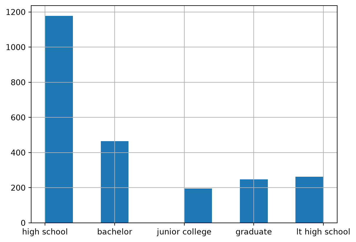
# For a simple histogram
my_data['degree'].hist()

# Standard Deviation
my_data['age'].std()

np.float64(18.06087856051088)

# Variance
my_data['age'].var()

np.float64(326.1953343775215)

# Compute the descriptive statistics of the wordsum variable.

# Obtain the frequencies of each gender(sex)

Multivariate Table

# To get a crosstab
my_cross_tab = pd.crosstab(my_data['degree'],my_data['marital'])

my_cross_tab

marital	1.0	2.0	3.0	4.0	5.0
degree
bachelor	231	35	75	10	113
graduate	142	17	34	4	50
high school	432	101	215	39	390
junior college	93	11	41	8	43
lt high school	100	36	38	14	74

# Do a cross-tabulation of sex and wrkstat

Appendix

Download a Copy of this Workbook

PythonI_Training.ipynb

Running R code in Jupyter notebooks

You can execute some R code inside a Python-based notebook. It is also possible to use Python code inside R-based notebooks. However, this should be minimized as much as possible as the underlying data and object structures are quite different.

This requires the rpy2 package (and a working R installation), which are not part of this workshop’s standard setup, so these cells are shown for reference but not executed.

# Activate R magic
%load_ext rpy2.ipython

%%R -i my_data

print(summary(my_data$age))
hist(my_data$degree)

The Zen of Python

import this

The Zen of Python, by Tim Peters

Beautiful is better than ugly.
Explicit is better than implicit.
Simple is better than complex.
Complex is better than complicated.
Flat is better than nested.
Sparse is better than dense.
Readability counts.
Special cases aren't special enough to break the rules.
Although practicality beats purity.
Errors should never pass silently.
Unless explicitly silenced.
In the face of ambiguity, refuse the temptation to guess.
There should be one-- and preferably only one --obvious way to do it.
Although that way may not be obvious at first unless you're Dutch.
Now is better than never.
Although never is often better than *right* now.
If the implementation is hard to explain, it's a bad idea.
If the implementation is easy to explain, it may be a good idea.
Namespaces are one honking great idea -- let's do more of those!