Stata I

Getting Started with Stata

After attending this training session, you will be able to:

1. Open Stata and existing datasets
2. Understand the layout of data
3. Obtain descriptive statistics and frequency tables
4. Transform a variable using generate and replace commands
5. Create graphs and edit them
6. Print output
7. Save and export output

Introduction

Code and Dataset

For this training session, please download the following data and code:

STATA workshop.dta

stata1workshop.do

What is Stata?

Stata is a menu- and syntax-driven statistical package. Most work can be done with simple Stata syntax.

Stata has these functions:

• Storing and organizing data
• Manipulating data
• Analyzing data using statistical procedures
• Graphing data
• Creating programs and macros

Stata comes with three versions, each with slightly different capacities in data management and data storage:

Small Stata

• Datasets restricted to approximately 300K bytes
• 99 variable (max)
• 1000 observations
• Slower than Intercooled Stata

Intercooled Stata

• 2,047 variables (max)
• Number of observations limited only by computer memory
• Maximum matrix size is 800x800
• String variables can only be 80 chars long
• Slower than StataSE

StataSE

• Maximum of 32,767 variables
• Number of observations limited only by computer memory
• Maximum matrix size is 11,000x11,000
• String variables can only be 244 chars long

Starting Stata

To launch the Stata program, open the Start menu (for Windows) or the Launch Pad (for Mac). Then search for STATA.

Stata Environment

By default, the Stata environment displays five windows: History, Command, Results, Properties, and Variables .

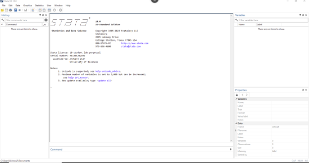
Command is a window where you can type, edit, and submit one command at a time.

Stata has the following keyboard shortcuts:

• Page Up: Steps backward through the command history
• Page Down: Steps forward through the command history
• Tab: Automatically completes a partially typed variable name

The History window shows the history of commands. It displays commands in black when successfully run and shows commands in red when incorrectly entered.

• Right-click in the Review window to Cut, Copy, Delete, Clear, or Save the commands.

• Double click on a command and this will rerun the command

• Commands can also be exported to a Do-file Editor by right-clicking and selecting Send to Do-file Editor.

The Results window (the window above the Command window) displays the results of statistical procedures, submitted commands, and error messages. By default, Stata displays the portion that could fit in the height of the Results window.

• If the length of the results exceeds the window height, Stata shows a message and will pause displaying the results.
• To display the next portion of the results, press the space bar or click on the go icon.
• To halt the procedure, press Ctrl-C or click on the stop icon.

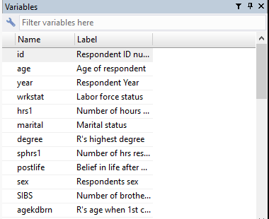
The Variables window shows the list of variables in current use and the Properties window shows the variable names, labels, storage types, and formats.

• To select variables, click on the variable of interest, and it will be copied into the Command window.
• Variable names, labels, and fonts can be changed in the data editor.
• To drop a variable from the data file, right-click on the variable and select Drop.
• Users can attach notes to variables and the data file in the data editor.

Opening an Existing Data File

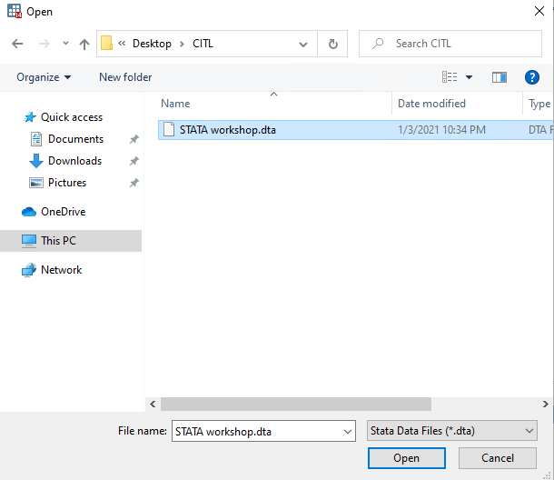
To open an existing data file, go to File > Open or click on the Open icon and select the drive or folder on which the data file is located.

Whenever you are unable to locate your data file, it is likely that the file is not in Stata format. Stata data files usually end in the suffix .dta so Stata looks for these kinds of files first. If the data file is in a different format, select All Files (*.*), and the file should appear. Double-click on the file, and Stata will open it if it is a type recognized by Stata.

Note

Changing the extension of a file to .dta does not magically make it into a Stata formatted data file. It must be imported through another program for Stata to be able to read it. Please contact us if you need assistance with this task.

What is the General Social Survey (GSS)?

The GSS is a demographic and opinion survey of U.S. households conducted by the National Opinion Research Center (NORC) at the University of Chicago. It has been collected annually or biannually (depending on the availability of funding) since 1972.

More than 38,000 respondents have answered over 3,000 different questions with regard to their opinions and attitudes toward economic, social, and political issues. It is well known for having the highest quality in overall survey design and is often used for examples in introductory statistics textbooks.

A subset of the 2018 GSS is used in this tutorial.

Stata Windows

In addition to the five basic windows described earlier, Stata has four areas that are tailored to specific needs.

Do-file Editor

The Stata Do-file Editor window is a syntax window where users can write multiple commands. To access it, click on the Do-file Editor button or go to Window > Do-file Editor > New Do-file Editor.

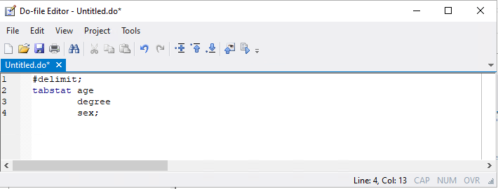
In the Do-file Editor, you can

• Highlight specific portions of code that you want to run, and perform those commands by clicking the Do button or going to Tools > Run.
• Type #delimit; before entering a command to tell Stata to read commands vertically.

Help Menu

Through the Help menu, you can search Stata topics such as basic language syntax, data management, statistics, graphics, programming, and matrices.

• Select Help > Search in the Main Menu toolbar, or type either help or help subject into theCommand window.
• The search results will be displayed in the Viewer window.

Viewer

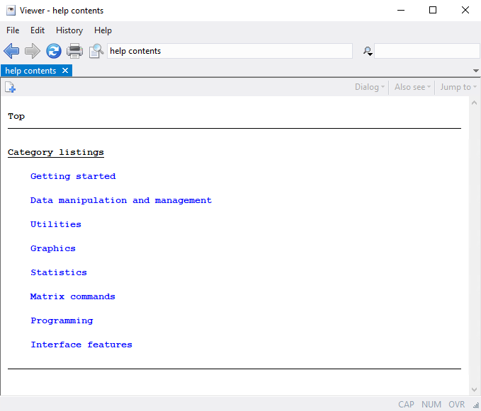
The Viewer window is similar to a web browser where you can search topics, find user-written programs, and install/manage third-party software.

• To receive recent information on Stata, click on the News icon in the help toolbar.
• To receive recent information on Stata updates, click on the What’s New icon in the help toolbar.

Log

A Log file is similar to a diary that records all procedures performed during a Stata session. The Log file will include the location and the names of data files used, commands, results, and error messages, but will not record graphic images.

1. To start a new log, go to File > Log > Begin and enter a file name to begin a log file saved in a directory of your choice. This log file will quietly record as you use Stata.

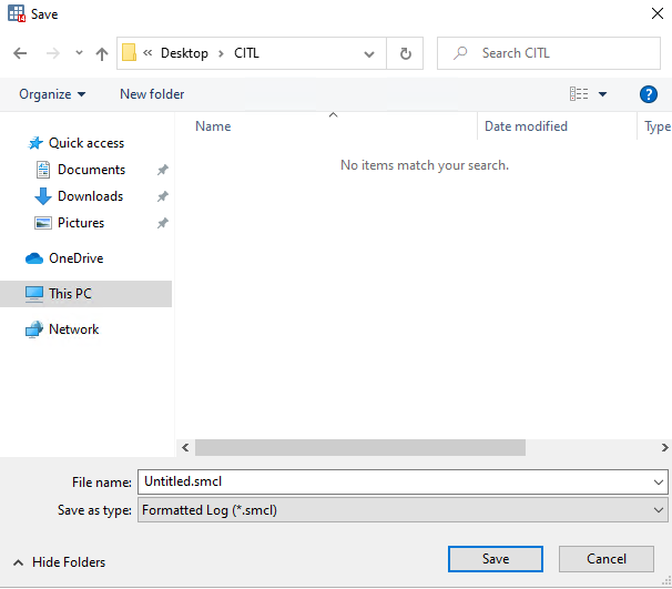
2. Select either Formatted Log (*.smcl) or Log(*.log) as a file type.

   • A Stata Formatted Log (*.smcl) can preserve fonts and color. This file type can only be opened with Stata.

   • A text (ASCII) log file (*.log) will contain only a plain text copy of the output. While this is a plainer output, .log is the recommended file name because you can open it in basic text editors on computers that do not have Stata installed.

3. Specify a file name and click Save. The Results window will display as below.

4. To close the log file, go to File > Log > Close.

Stata displays the status of a log file in the Results window as well as at the bottom right-hand corner of the window.

Opening, Appending, and Overwriting Existing Log Files

1. Go to File > Log > Begin, and select the log file that you wish to open.
2. Click Open. This will launch the Stata Log Options dialog box.
3. Select how you would like to open the file, and click Ok.

Data Editor

The Data Editor window is similar to a spreadsheet in Excel, SPSS, or SAS where users can input new data, edit existing data, and sort both new and existing data.

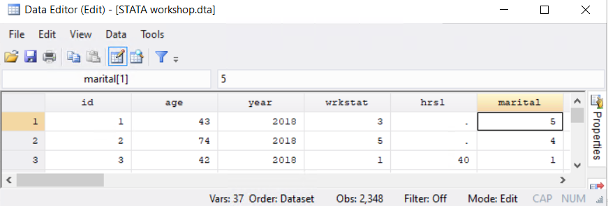
The data editor can be opened in three ways. To open the Data Editor, you can click on the Data Editor button, go to Data > Data Editor > Data Editor (Edit), or go to Window > Data Editor. After you have finished editing, you can save the changes by clicking on Save button.

The Data Editor is divided into many individual boxes (i.e., cells), and these cells are arranged into rows and columns. Each row is labeled with a number, and each column is labeled with a variable name.

More specifically, each row displays a case, and each column contains a particular variable. A case may be an individual person, a single country, or any other unit of analysis for which data has been collected.

Imagine, for example, that the data comes from a poll or survey. Each row represents an individual person who participated in the poll, and each column represents the answer to a question that was asked of that person.

This row-by-column arrangement is the most typical way to organize data in the social sciences.

Sorting Variables in Alphabetical Order

Warning

Stata does not have an option to bring back the original order of the variables once they have been sorted by alphabetical order. If you wish to revert to the original order of the variables, close the file without saving, and reopen it.

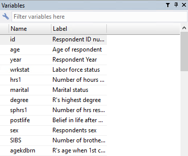
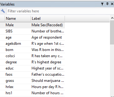
By default, the Variables window displays variables in the order that they appear in the file, meaning that the data are not necessarily sorted in an alphabetical order. In Stata 18, the command order is the command you will input in order to reorder your list of variables. The aorder command from past versions of Stata is no longer extant. More information on order can be accessed with help order. You can move variables to the top or the bottom of the file or order the data alphabetically. To move a variable to the top of the list, use order varlist, first. To move a variable to the bottom of the list, use order varlist, last. Most people are interested in an alphabetical order. Rather than specifying variable names, to order all your variable names use order _all, alpha or order _all, seq. Note that the variables with capital letters will be ranked on top.

Before order_all, alpha

After order_all, alpha

Viewing the Content of Data

There are two ways to view the content of a data file in current directory: describe and codebook.

The Describe Command

The describe command gives the descriptions of a data file and variables, including the location of the file, the total number of observations, the total number of variables, and the size of the data file.

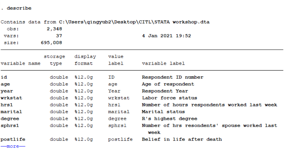
The first line shows the location of the data file. This data, for instance, is saved under the C:\ drive, and the file name is STATA workshop.dta. The second line shows the number of observations, and the third line tells you the number of variables stored in the dataset. This dataset includes 2,348 observations and has 37 variables. The latter part of documentation shows you how to attach value labels or variable labels to a variable.

The describe command can also be combined with more options. For instance, describe varName will display a description of the variable specified. Here is the description of the variable age using the below code:

describe age

• Variable name shows the internal variable name in Stata. In other words, if you wish to use the variable in your analysis you will need to use this name in the command box.
• Value label shows which value label is attached to a variable. Value labels may be up to 32,000 characters long.
• Variable label shows you a longer description of the variable and allows for more flexibility. For example, you may use quotes and spaces in the variable label. People often use the question wording from a survey in the variable label.

The Codebook Command

The codebook command is similar to a diagnostic tool that examines variables in a data file for potential problems, lists the descriptions of variables as well as missing values patterns, and prints notes attached to the data file, including the date and the person who last saved the data file.

To get a snapshot of a data file use:

codebook, compact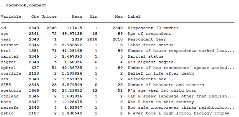

Note

Here, the compact option tells Stata to display the output in a compact row format. Without this option, Stata would generate a separate table for each variable.

Each row represents information on the variable. For instance, the second line is the information for the variable age:

• The number of observations is 2341.
• The number of unique values is 72.
• The mean age is roughly 48.97.
• The youngest age is 18.
• The oldest age is 89.
• The label is “Age of respondent”.

The option problems shows the potential problem(s) found in a data file:

codebook, problems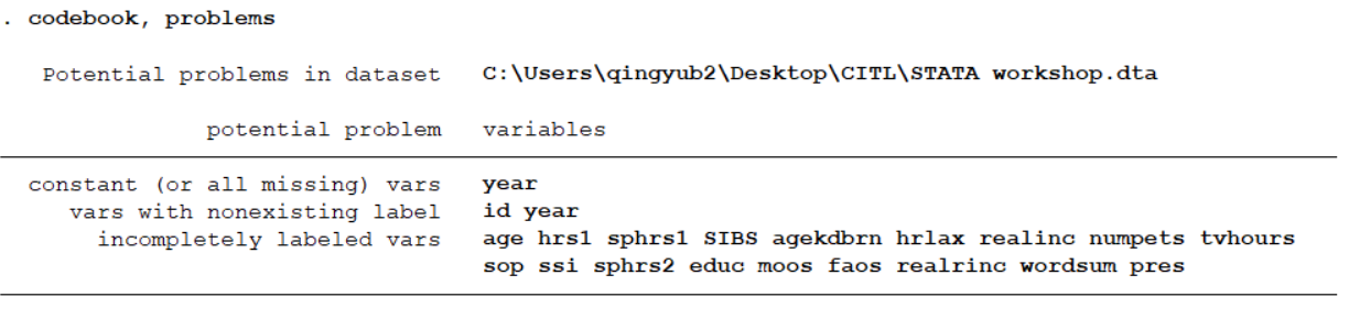

The option mv searches the data to determine the patterns of missing values. Here is what it found on the variable grass:

codebook grass, mv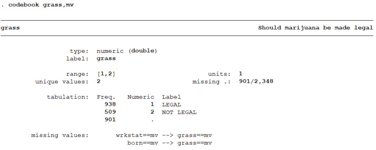

A period (.) in the tabulation list indicates missing values. As you can see from the output, if a case does not have a value for wrkstat, it does not have one for grass either.

Descriptive Statistics

Summary Statistics

The summarize varName(s) command calculates and displays univariate summary statistics for the variables listed. If no variable list is specified, then summary statistics are calculated for all the variables in the dataset.

The detail option produces additional statistics, including skewness, kurtosis, the four smallest and largest values, and various percentiles (including the median = 50%).

summarize age, detail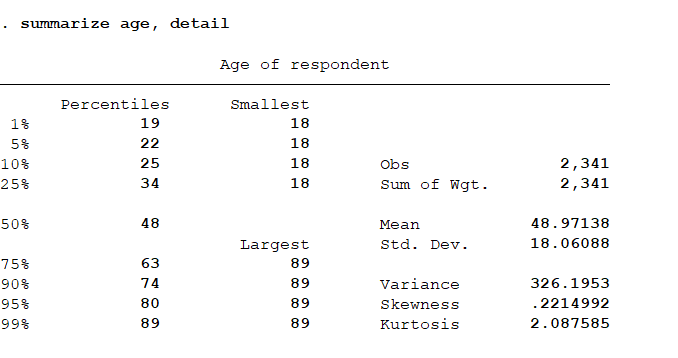

Frequencies

The tabulate varName command generates a frequency table illustrating how cases are distributed across the values of a variable.

For example, a frequency table for the variable degree (a respondent’s highest degree) will show you how many respondents have “less than high school,” “high school,” “junior college,” “bachelor,” or “graduate” levels of education in the data file using this code:

tabulate degree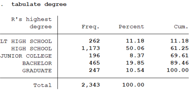

b7_tabulate

The first cell in the first row shows a variable label “LT HIGH SCHOOL” and then displays the frequency (262), percentage (11.16), and cumulative percentage (11.16), respectively. That is, the number of respondents who have completed less than high school is 262, which constitutes 11.16% of the total respondents. Likewise, the first cell in the second row shows a variable label “HIGH SCHOOL” and then shows the number of respondents who completed high school but no further education (1,173) and the percentage (50.06) of the total respondents. The cumulative percentage is 61.25, because it is a sum of 11.16% and 50.06%.

Note: tabulate ignores missing values unless explicitly indicated by the missing option. When this option is specified, missing values will be reported as the last row of the table generated, signified by a period (.). Example code:

tabulate degree, missing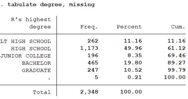

The frequency table generated using the missing option displays descriptive statistics for the variable degree with the addition of missing values into the table. The total number of cases in the first frequency table is 2,343, while the second table has 2,348 cases as the grand total, because the latter includes 5 missing values (.).

Exercise 1

Run a table and summary statistics for the variable SIBS, number of brothers and sisters.

• What is the total number of cases?

• What is the number of missing cases?

• What is the mean, the median, range, and standard deviation of SIBS?

See Appendix A for answers.

Data Transformation

Recode

The recode procedure changes, rearranges, or consolidates the values of an existing variable.

Sometimes you will need to recode a variable into a new variable by combining responses into a smaller number of response categories. For instance, look at the variable wrkstat using the code:

tabulate wrkstat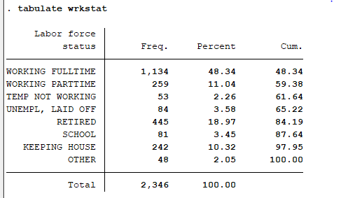

Say we wanted to create a new variable that captures the respondent’s labor force status; either they are part of the labor force (“Working full time”, “Working part time”, or “Temporarily not working”) or they are not (all other values). To do so in Stata we need the numeric values that correspond to the character values that we have above. We can see these numeric values by including the nolabel option in our tabulate command. Let’s also include missing to get an idea of the number of missing cases we have:

tabulate wrkstat, missing nolabel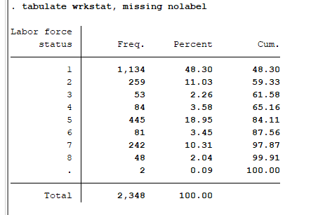

To get the new variable we want we need to combine values 1 through 3 into “In the labor force” and 4 through 8 into “Not in the labor force”.

The default setting for recode is to overwrite the original variable. If we want to keep the original variable we can include the generate command. This will write our recode into a new variable with the name given in the paraentheses.

recode wrkstat 1/3=1 4/8=0, generate(wrkstatRecoded)

The syntax works as follows: after the command name we have the variable that we want to recode, followed by the first value for the new variable. This is written as first old value/last old value = new value. We repeat this syntax for the second value.

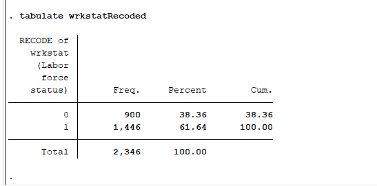
The new variable will appear at the bottom of the Variables window. By default, Stata attaches “Recode of oldvar” as the label for the new variable, in this instance “Recode of wrkstat”. You should compare the values of the old and new variables to ensure that the values were recoded correctly by using the tabulate procedure presented earlier in this document such as:

tabulate wrkstat
tabulate wrkstatRecoded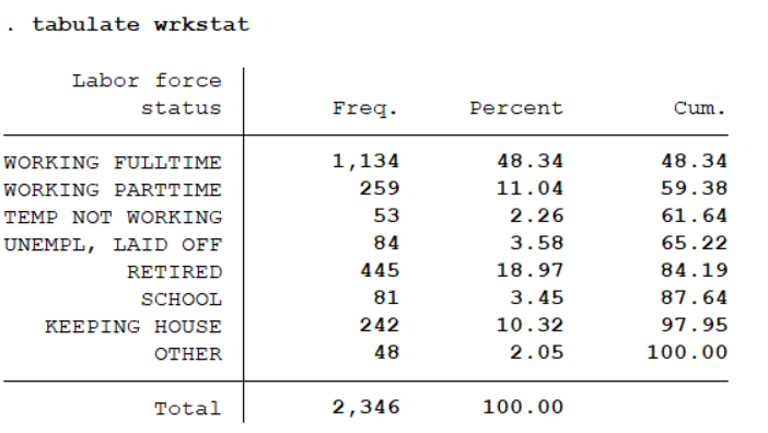

Some recoding examples:

Command	Result
recode x 1=2	Equivalent to replace x=2 if x==1 (CONFUSING?)
recode x 1=2 3=4	Changes 1 to 2 and 3 to 4 in x
recode x 1=2 2=1	Interchanges 1 and 2 in x
recode x 1=2 2=1 \*=3	Interchanges 1 and 2 in x and changes all other values to 3
recode x 1/5 = 2	Changes values 1 through 5 to 2 in x
recode x 1 3 4 5 = 6	Changes values 1, 3, 4, and 5 to 6 in x
recode x min /5 = min	Recodes the minimum of x through 5 to the minimum of x
recode x 6/max = 3	Recodes t through the maximum of x to 3 in x
recode x . = 9	Changes mixxing values of x to 9

Labeling Variables

Value labels are convenient ways to connect otherwise unintelligible values in data to short interpretable phrases.

Two steps are needed to set a variable’s value label: (1) create a value label, and (2) attach the value label to the variable.

First, we need to create a value label that we then will assign to our varaible. Defining a value label requires us to identifiy the existing numerical values and that then assign the label we want to it. To define the label, wrkLabel, type:

label define wrkLabel 1 "In the labor force" 0 "Not in the labor force"

Note

The label has not been applied to any variables yet, so if you tabulated wrkstatRecoded, the table would still only report the values.

To apply the label to the values of wrkstatRecoded, type:

label values wrkstatRecoded wrkLabel

Now the tabulate output will display the value labels when we use the code:

tabulate wrkstatRecoded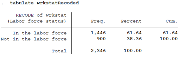

In summary, to apply a label to data, variables, or variable values:

• label data “text for label”
• label var variablename “text for label”
• label values variablename “labelname”

To change a value label, first you need to delete the entire label and then redefine it, including all its values:

• label drop labelname
• label define labelname value “text for label” …

Creating a New Variable

The generate command creates new numeric variables or modifies the values of existing string or numeric variables. This command will create a new variable in the data set while leaving the original variable unchanged.

For example, to create a new variable that adds the number of hours the respondent worked last week, variable hrs1, and the number of hours the respondent’s spouse worked last week, variable sphrs1:

generate totalHourCouple = hrs1 + sphrs1

Note

Stata does not automatically overwrite existing variables. If you want to use the same variable name, then the variable needs to be dropped and then computed using the new criteria. You can also use the replace command.

We can check that our new variable has been created using tabulate:

tabulate totalHourcouple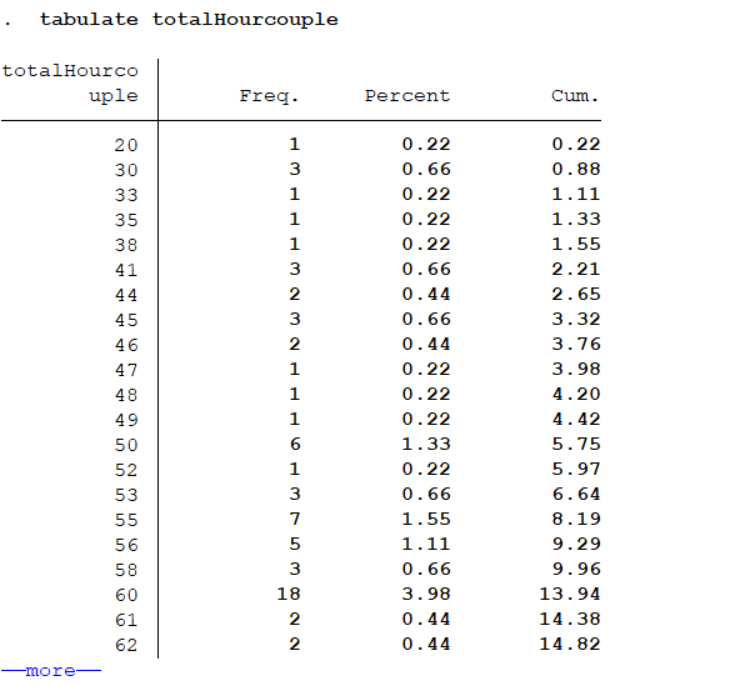

Click more to display missing values

The new variable totalHourCouple has 1,896 missing cases. But if you run tabulate on variable hrs1 and variable sphrs1, you will get 967 and 1,711 missing cases respectively.

The disparity in the number of missing cases occurs because all cases with at least one missing value in either hrs1 or sphrs1 will be given a missing value for the new variable.

Arithmetic	Logical	Relational
+ addition	~ or ! not	> greater than
- subtraction	| or	< less than
* multiplication	& and	>= greather than or equal
/ division		<= less than or equal
^ power		== equal
+ string concatenation		~= or != not equal

Exercise 2

To practice the recode and generate commands:

Let’s say that we wanted a new marital variable capturing if the respondent had ever been married or not:

1. Create a new variable that recodes NEVER MARRIED into 0 and the others to 1.

2. Label the new variable values as 1= “Has been/is married” and 0 = “Has never been married.”

See Appendix A for answers.

Multivariate Tables

Contingency Tables

The tabulate command produces contingency tables, also know as crosstabs, showing the joint distribution of two or more categorical variables.

In contingency tables, the frequency distribution of one variable is subdivided according to the values of one or more other variables. The unique combination of values for two or more variables defines a cell.

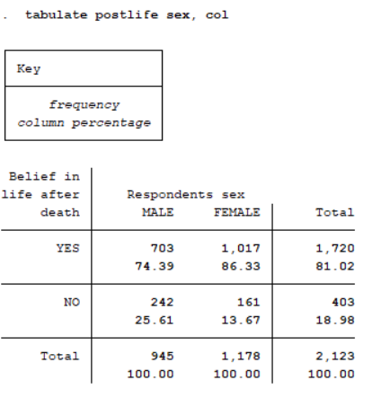
For example, to run a two-by-two table of postlife and sex, type:

 tabulate postlife sex, col 

The general format is as follows: tabulate rowVar colVar, options

Note

The col option tells Stata to include column percentages in the output. When creating crosstabs, you always want the percentage of the independent variable. Because sex is the independent variable, we have specified that as our column variable and requested column percentages.

Interpretation of Crosstabs Output

From the output produced once the command has finished, we can see the following:

1. Number of valid cases: 2,123 cases are included in the crosstabs table.

2. 74.39% of male respondents believe in life after death

3. Combining male and female, 81.02% of respondents answered “believe in life after death.”

Note

Only valid values are included in the crosstabulation table. Thus, a case with a missing value for at least one of the variables will be excluded from the table.

Exercise 3

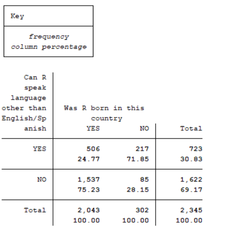
Find out how many foreign-born and native-born survey respondents can speak a language other than English/Spanish. That is, run a crosstab using variables othlang (Can respondent speak a language other than English?) and born (Was respondent born in this country?). See Appendix A for answers.

Graphics

The following will show you how to produce charts in Stata. Please note that charts in Stata are not displayed in the Results window. Rather, a Graph window will appear. Once you close this window, your graph will be lost so if you wish to use the graph later you will have to save it by selecting File > Save As… in the Graph window.

Bar Chart

A bar chart is a graphic representation of numerical values of a categorical variable, which uses rectangles to show a frequency or a proportion of each category in the variable. Spaces are inserted between each rectangle in order to differentiate a bar chart from a histogram. Histograms are graphic representations of continuous variables and as such, have no spaces between each rectangle.

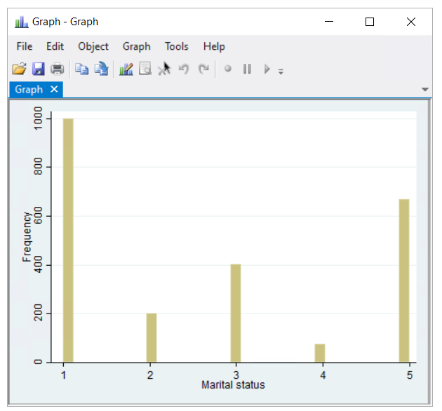
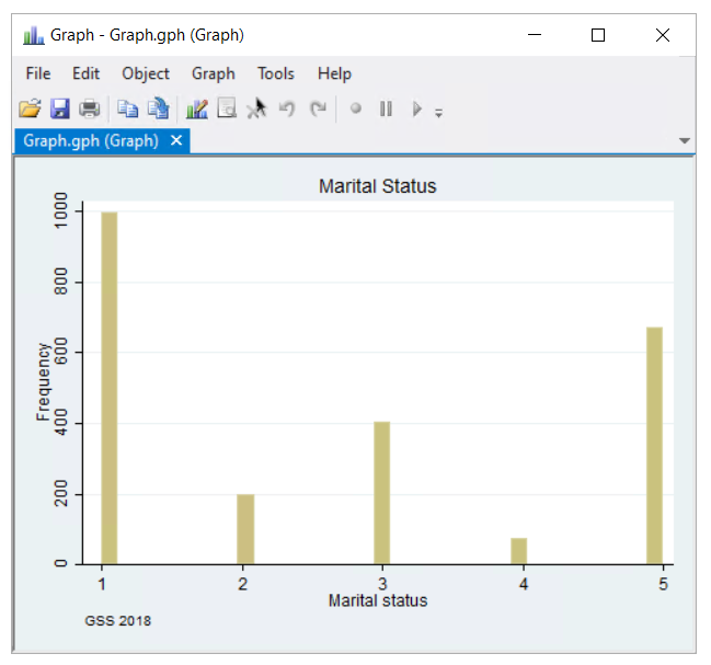
To create a bar chart for the variable marital (marital status), use the command:

histogram marital, frequency

Note

Even though the command says histogram, the resulting chart is indeed a bar graph because the variable represented is a categorical variable (not continuous) and has spaces between each rectangle.

d1_bar

Editing a Chart

By default, Stata displays the labels for y- and x- axes. Submitting additional options is required to insert a title, note, legend, etc.

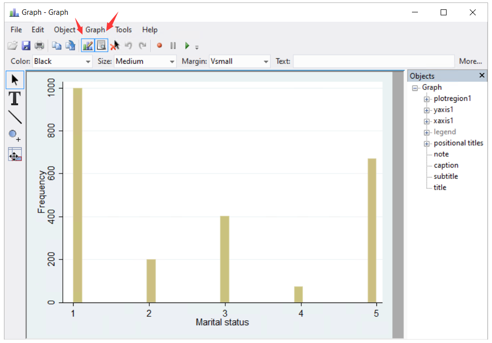
The Graph Editor is an alternative to writing option commands. It allows you to add, modify, and remove texts, reference lines, grids, and miscellaneous formats.

To open the Graph Editor, select File > Start Graph Editor in the Graph window or select the Graph Editor button in the toolbar. This will launch an Object Browser pane.

Should this pane not appear once you start the Graph Editor, you can enable it by pressing the Object Browser icon in the toolbar.

Adding a Title

1. In the Object Brower window, select positional titles > top1.
2. This will launch the Textbox properties dialog box. Type “Marital Status”, and change the text style, if necessary.

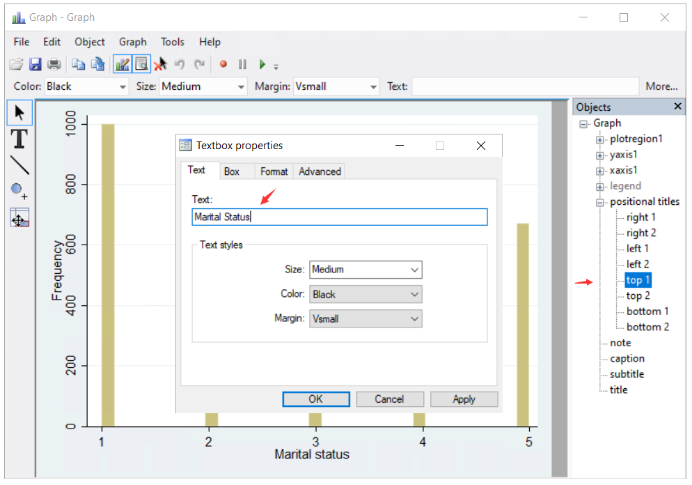
3. Once you are done making your changes, click OK to finish.

Adding a Footnote

1. In the Object Brower window, select positional titles > note.
2. This will launch the Textbox properties dialog box. Type “GSS 2018”, and change the text style, if necessary.

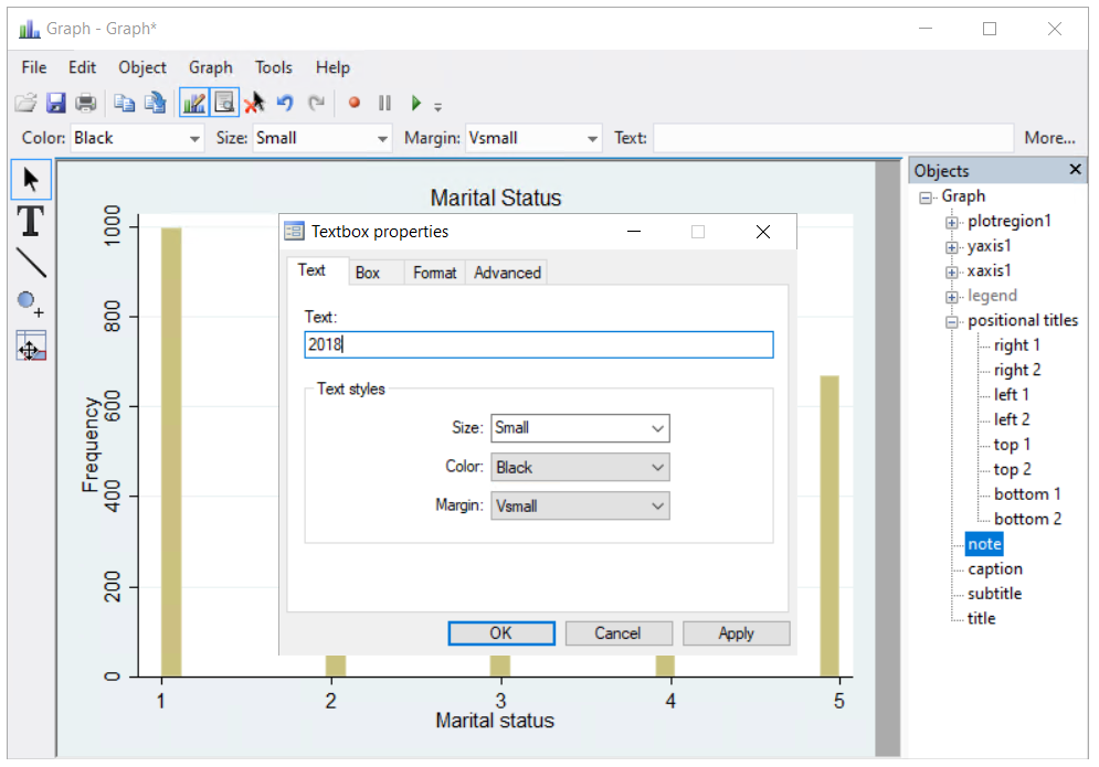
3. Once you are done making your changes, click OK to finish.

Here is the resulting chart:

Pie Chart

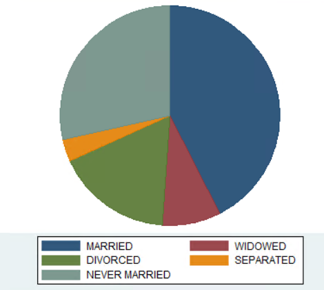
A pie chart is a graphic representation of a categorical variable, which uses a slice in a circle (or a pie) to show a frequency or a proportion of each category in the categorical variable. It is typically used to compare proportions. For example, a pie chart may be used to illustrate the proportional distribution of marital status.

To create a pie chart for the variable marital (marital status):

graph pie, over(marital)

Below shows a pie chart with the default format

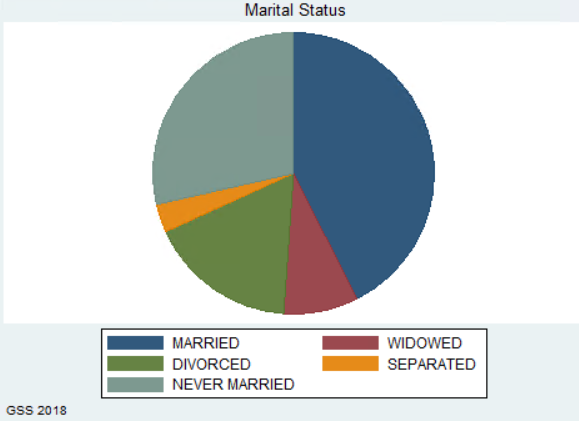
And one after editing the title and footnote in the Graph Editor.

Adding a Grouping Variable

To add a grouping variable (i.e., sex), use the by() option. For example, to create pie graphs to display the proprotional distribution of marital status by sex:

graph pie, over(marital) by (sex)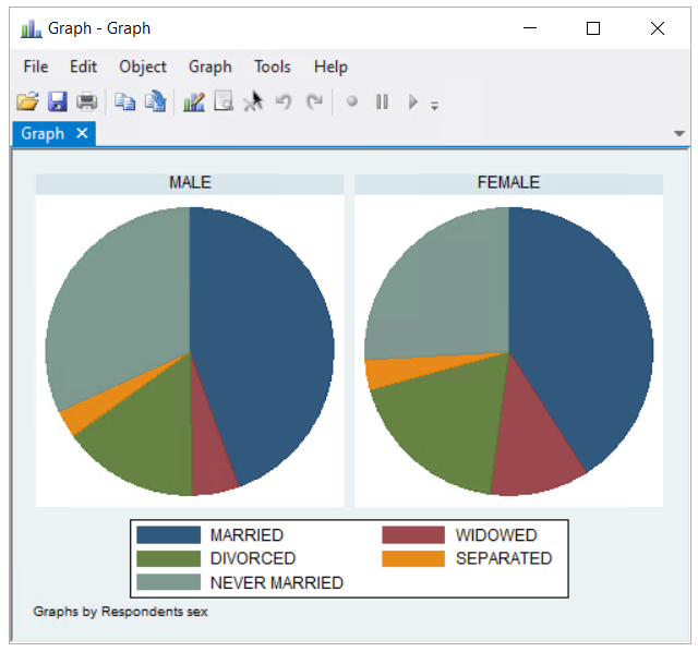

Exercise 4

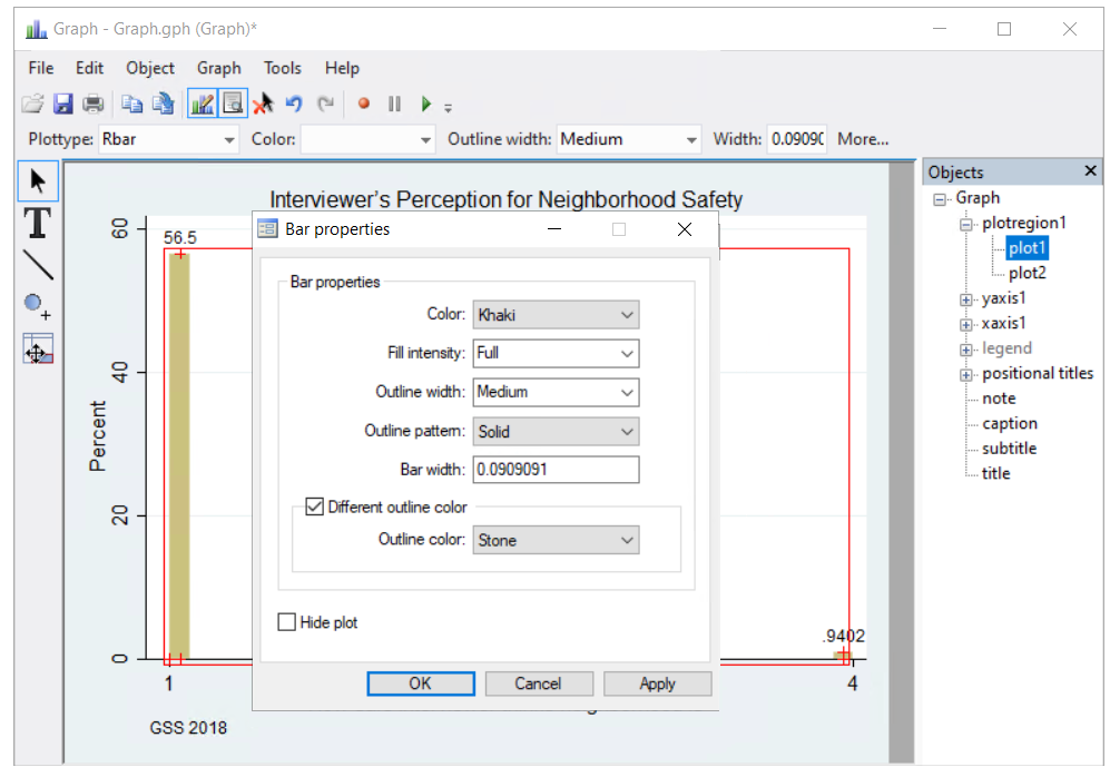
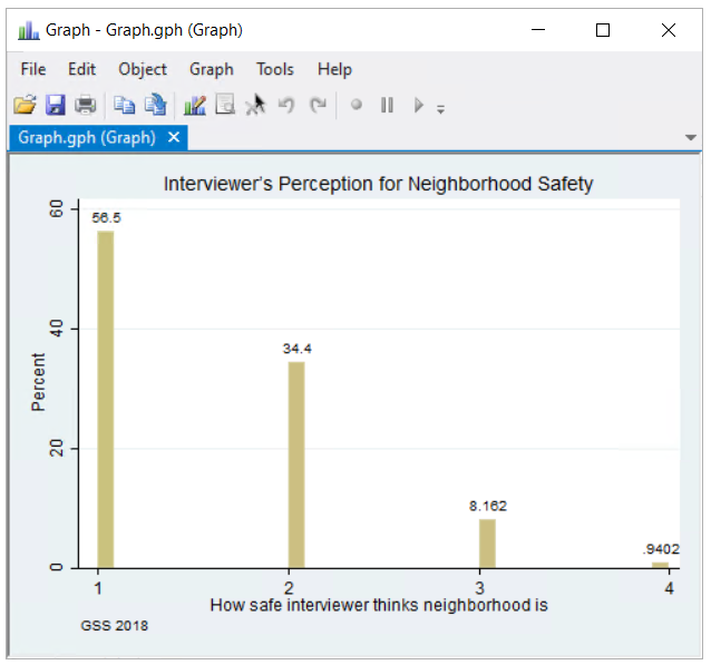
Create a bar chart for the variable neisafe. This variable is based on the question, “How safe interviewer thinks neighborhood is?” The answers are categorized as: Very Safe, Somewhat Safe, Somewhat Unsafe, Very Unsafe.

• Display the data labels for each bar (in percent). What is the percentage for “Very Safe”?
• Include the title”Interviewer’s Perception for Neighborhood Safety” and footnote “GSS 2018”.
• Can you change the fill color of the bars and the width between bars?

See Appendix A for answers.

Saving and Printing

Saving your Data and Output

The easiest way to save your data is to click on the Save button.

If you want to save a new dataset:

1. Select File > Save as….
2. In the Save Data Files dialog box, specify a file name and file location.
3. Leave the extension as .dta, the Stata data format, and click Save.

Printing from Stata

There are several ways to print results from Stata. First, you could print from a log file, which can capture commands and results. Otherwise, simply right-click on the display window and click on the option Print, following the usual guidelines. If you have a .pdf writer installed as a printer driver (which can be done with a program such as CutePDF), you can print to the .pdf driver as well.

Important

We recommend that you create a log file at the beginning of your Stata session, because results are only saved to the log file after you create it.

Printing Logs

You can print a log file by clicking on the Print button. However, you cannot delete portions of the log file without translating it to a text file or copying the output into a word processor.

To print a log file from the Viewer during a Stata session:

1. Click on the Print button. This will launch the Print dialog box.
2. If you wish to change the printing settings, click on Preferences.
3. Once finished changing your settings, select OK to go back to the Print dialog box. 4. Select a printer, and click Print.

To print a closed log file, you must first open it.

1. Select File > View….
2. Enter a filename, and click OK.
3. Then print the log file according to the above instructions.

If your log file is a plain text file, you can open it in any text editor (like Notepad), the Do-file editor in Stata, or a word processor. From within your editor or word processor, you can edit and print it.

Note

If your log file is a .smcl file, you need to translate it into a text file. Make sure that you have closed the log file before conversion.

1. Select File > Log > Translate. This will launch the Translate File dialog box.

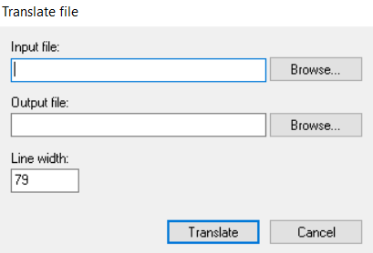
2. Click on the Browse… box for Input file:, and select the file you want to translate.
3. Then, click on the second Browse… box for Output file:, and select the place where you want to place the new file.
4. Type in the new file name and the extension for the text file, and click Save.

Tip

Your world processor will initially display the file in its own default font. The log file will not be very readable when printed in a proportionally spaced font (e.g. Times New Roman or Helvetica). It will look much better printed in a text-width (“typewriter”) font (e.g., Courier).

Appendix A: Answers for Exercises

Exercise 1

To find out the number of total and missing cases, type:

tabulate SIBS, missing

Output:

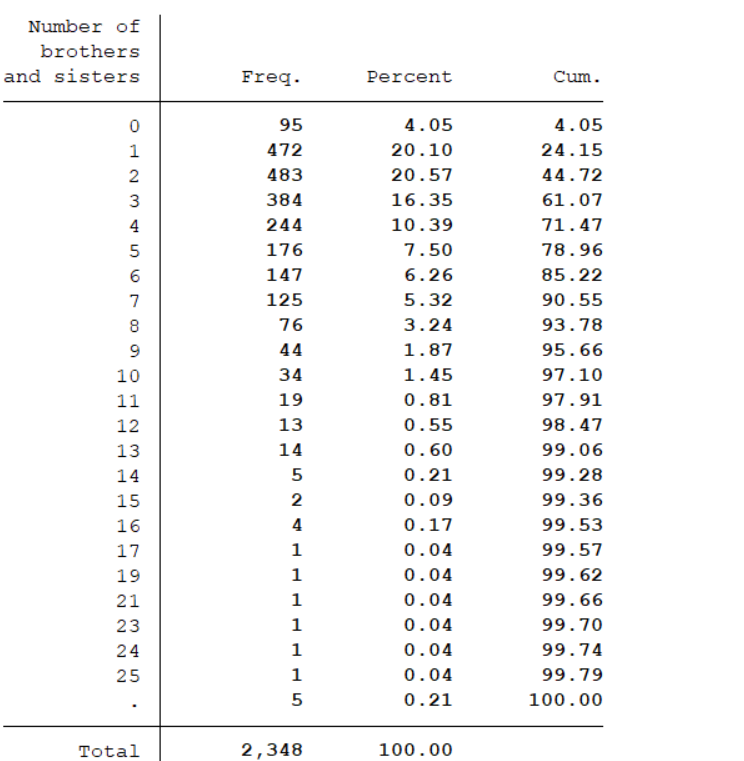
Interpretation:

• There are 2,348 total cases.

• There are 5 missing cases.

To find out the number of valid cases and the descriptive statistics for sibs, type:

summarize SIBS, detail

Output:

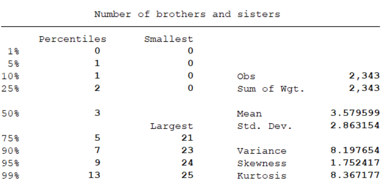{fig=alt=“Detailed summary including missing values for SIBS variable”}

Interpretation:

• There are 2,343 valid cases.
• The mean is 3.579.
• The median is 3.00.
• The range is 25.
• The standard deviation is 2.863.

Exercise 2

Create maritalRecoded

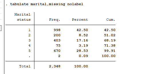
First look at the marital variable, with and without labels:

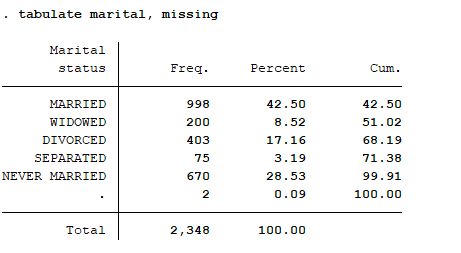
tabulate marital, missing
tabulate marital, missing nolabel

2. Create a new variable that recodes NEVER MARRIED into 0 and the others to 1.

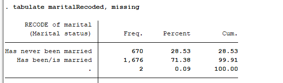
recode marital 1/4=1 5=0, generate(maritalRecoded)

3. Label the new variable values as 1 = “Has been/is married” and 0 = “Has never been married.”

label define maritalLabel 1 "Has been/is married" 0 "Has never been married"
label values maritalRecoded maritalLabel

Output:

label_maritalRecode

Exercise 3

To create a crosstab of othlang and born, type:

tabulate othlang born, col

Output:

Interpretation:

• Number of valid cases: 2,345 cases are included in the crosstabs table.
• 24.77% of native-born respondents answered yes, they speak a language other than English/Spanish.
• Combining native- and foreign-born, 30.83% of respondents answered yes, they speak a language other than English/Spanish.

Exercise 4

To create a bar chart of neisafe which displays the percentage of each category, type:

histogram neisafe, percent addlabels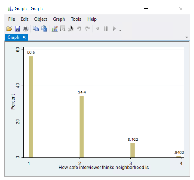

To add the titles and footnote:

1. In the Graph window, select File > Start Graph Editor.
2. In the Object Browser window, select positional titles > top1.
3. Type “Interviewer’s Perception for Neighborhood Safety”, and click OK.

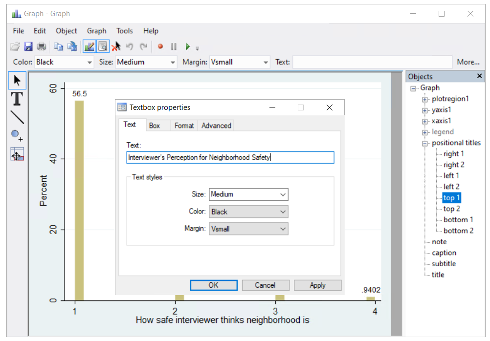
4. In the Object Browser window, select positional titles > note.
5. Type “GSS 2018”, and click OK.

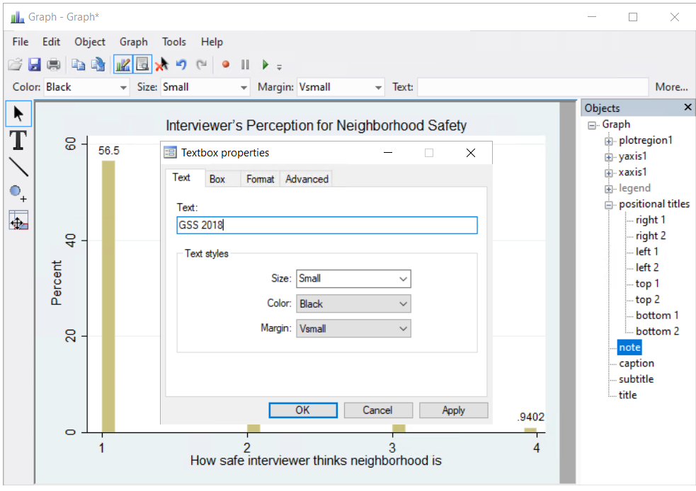
Result:

To format the chart colors:

1. In the Graph window, select File > Start Graph Editor.
2. In the Object Broswer, double-click plotregion1.

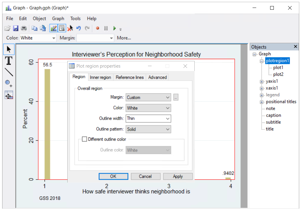
3. To change the background color of the graph, go to Color: and select a color from the drop-down menu.
4. To change the margin, go to Margin: and click More… for more options, or double-click the graph to launch the Plot region properties dialog box.
5. To change the color or format of a bar, double-click the bar in the graph or select plo1 in the Object Browser under plotregion1, and the Bar propertites dialog box will appear.