R I

Getting Started with R

After attending this training session, you will be able to:

1. Use Basic R syntax
2. Use Common R packages
3. Import datasets from other software such as SPSS, EXCEL, and Stata
4. Compute new variables and recode variables
5. Create frequency and contingency tables
6. Obtain univariate statistics
7. Create graphics and charts
8. Save and export output

Introduction

Code and Dataset

For this training session, please download the following data:

R_Data.csv

What are R and RStudio?

R is statistical software that is licensed as an open source program under a GNU license. In other words, it is free. As statistical software, it can be used for data manipulation, calculation, inference, and graphical display. It contains advanced statistical procedures sometimes not available in other statistical software. It is available on Windows, Linux, and Mac, and can be downloaded for free at https://cran.r-project.org/.

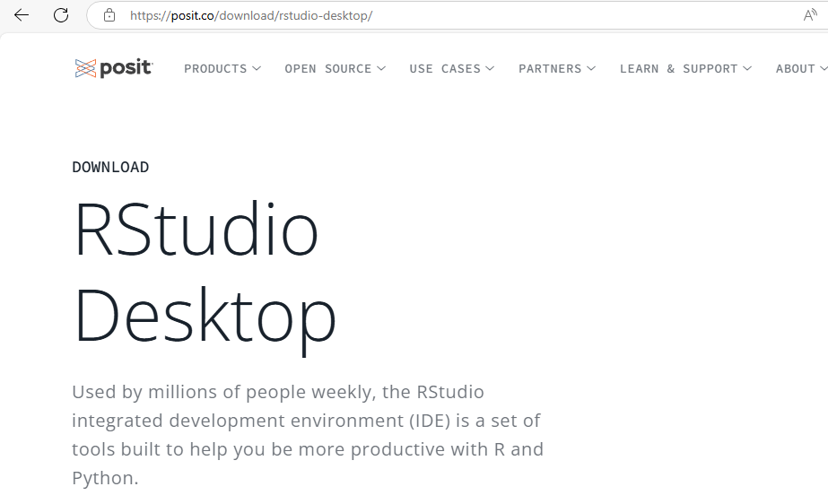
RStudio is a user interface for using the R statistical programing language. We highly recommend using RStudio (or another program like Positron, but we will only cover RStudio today). RStudio and R are both free for download from the Posit website https://posit.co/download/rstudio-desktop/.

To use RStudio, you must first also install R on your computer. In the next section, we will navigate through the RStudio environment.

What is the General Social Survey (GSS)?

The GSS is a demographic and opinion survey of U.S. households conducted by the National Opinion Research Center (NORC) at the University of Chicago. It has been collected annually or biannually (depending on the availability of funding) since 1972.

More than 38,000 respondents have answered over 3,000 different questions with regard to their opinions and attitudes toward economic, social, and political issues. It is well known for having the highest quality in overall survey design and is often used for examples in introductory statistics textbooks.

A subset of the 2018 GSS is used in this tutorial.

Starting R / RStudio

To launch RStudio, click on the start icon in the lower left-hand corner of the screen. Select RStudio from the list of programs.

RStudio Environment

The RStudio environment consists of four basic elements by default: the Script Editor, the Console, the Workspace pane, and the Viewer.

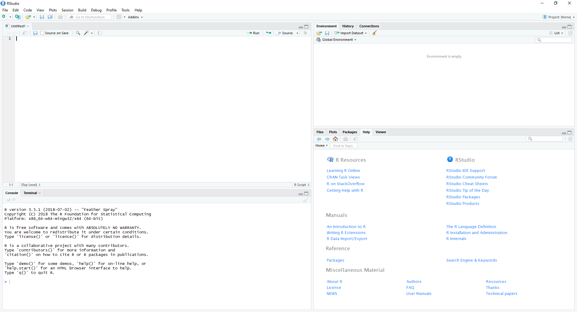
The Menu Bar has pull-down menus that when clicked will display additional commands.

R Console vs. Script

Console

The R Console window can be used to enter commands and view printed results or messages (errors, warnings, information, etc.).

R has a built-in command-line calculator, which is useful for quick math functions and data transformations that you don’t want to save in a script.

Go to the R Console command line and type in a basic mathematical function, such as 10-8, 23*2, 5/5 or log(90).

After each function, press ENTER.

The results should appear as below:

> 10-8
 [1] 2
> 23*3
 [1] 69
> 5/5
 [1] 1
> log(90)
 [1] 4.49981

Scripts

Several commands at once can also be written in the R Script Editor and then submitted. In an R session, you cannot save commands written in the console. You can use ↑ and ↓ on the keyboard to cycle through previously entered commands. Sometimes, you will need to perform a fairly complex analysis that consists of a series of commands. In such cases, you will want to write your commands in the script editor so that you can save it for future review or to re-run the commands at a later time.

To create a new script in RStudio, click on the New File button in the upper left hand corner of RStudio. Then click on R Script to create a new empty R Script.

A green plus icon for creating new files is visible.

In R, any lines beginning with # are treated as comments.Commented lines are useful for adding descriptive information to your code.R will not run any code in a line after a pound sign.See the example below:

# This opens the R help documentation
help.start()

To execute a command written in the Script Editor, place the cursor on the command line, and then type Ctrl + Enter (Cmd + Enter on Mac). The executed command will also appear in the R Console.

To run multiple lines of script at once, highlight the desired lines and use the same command.

To save the script, click File > Save as... or press Ctrl + S (Mac: Cmd + S).

Workspace and Viewer Panes

Workspace Pane

The Workspace consists of all of the objects defined by the user.

In RStudio, a summary of the objects in memory will be displayed in the Environment tab of the Workspace pane. This may consist of data frames, lists, vectors, or other objects.

Data frames and lists can be previewed in the Environment tab by clicking on the triangle next to the object name. This will display information about the variables in the data frame, such as name, object type (numeric, factor, etc.), and the first values. The number of variables and observations are also listed next to the name of the data frame.

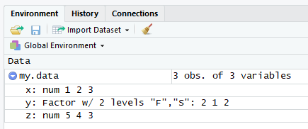
If you want to remove objects from your workspace environment, you can do so using the code remove(list="my.data"), where my.data is the name of the object you want to delete. You can also remove all objects at once by using the coderemove(list=ls()).

Also, note that in RStudio, data can be loaded by clicking on Import Dataset in the Environment tab of the Workspace pane. Code for loading the data set is recorded in the Console and History.

In the History tab of the History/Environment pane, a list of all the commands entered are displayed. Double clicking on a previous command automatically sends the command to the console.

Viewer Pane

In the Viewer pane, you will be able to search for files, display information about R packages, and explore help pages. Some outputs from the Console, such as graphs, plots, and help requests, will be displayed here as well.

To become familiar with how the Console and the Viewer pane interact, let’s submit a help request, typing ?plot.

Remember to press Enter to execute a typed command (or Ctrl+Enter if working in the Script Editor). Information about the plot function should be displayed.

Now let’s display something in the Plot tab of the Viewer pane.

In the script editor (or in the console), type:

x = c(1:6) # defining the vector, x
y = x + runif(6) # defining the vector y as a function of x
            # and random draws from the uniform distribution
plot(x,y)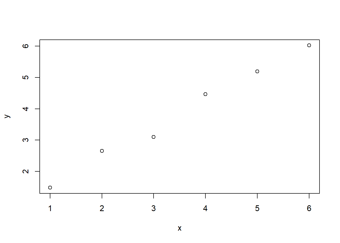

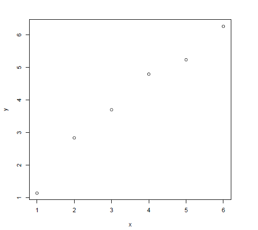
You will see the plots in the lower right hand pane, with the Plot tab activated.

If you click on the Help tab, you will see the last help topic.

General Tips for Console

There are a few tips to keep in mind when using the Console:

• R commands are case-sensitive. If you accidentally type and submit Help.start() instead of help.start(), you will get an error message stating that R could not find that function.
• > is the R prompt. If you do not complete a command, you will see + at the end of a line. To complete the command, just add the remaining element of the command directly after the + sign.
• Different commands are generally typed in a new line. If you wish to execute two or more commands simultaneously, enter them in the same line, each separated by a semicolon (;). Example: print("hi");print("bye")
• Single quotation marks or double quotation marks are used interchangably – but should be used consistently.
• ↑ (Up Arrow) steps backward through the command history and ↓ (Down Arrow) steps forward through the command history.
• TAB automatically completes a partially typed variable name or function; it can also prompt function arguments.
• Ctrl+L will clear the R Console. This will not delete objects in the environment (in memory).
• The ESC key will stop the execution of a command.
• Some function arguments require quotation marks and others do not. For example, typing install.packages(spdep) instead of** install.packages("spdep") will return an error. Check the syntax for the function you are using.
• Incorrect use of slashes can be common source of errors in R. For example, in Windows, you must use setwd("c://mydata") instead of setwd("c:\mydata").

Packages and Library

R is equipped with a standard set of packages. The primary contents of packages are functions and data. The library is the directory where packages are located. In addition to the standard set of packages, many other packages are available for download and installation. The number of R packages is constantly increasing due to many contributors within the R community. Additional R packages may be used for a specific statistical analysis that otherwise is impossible or much harder to do with standard R packages (for example, spatial analysis) or can have other functions such as creating more attractive and flexible plots. In short, adding other packages allow us to perform a greater variety of types of analysis.

To install a package, use the command install.packages("packagename"). Try to install the package foreign. You generally only need to install packages once on a computer.

Once packages are installed, they need to be loaded each time you want to use them in an R session. You can load packages by typing library(packageName) (e.g. library(foreign)). We recommend loading packages all at once in the beginning of your R script.

Once a package is loaded, more information about the package can be obtained by typing library(help=packageName) or by searching for or locating the package under the Packages tab of the Viewer pane. Continuing with our foreign package example, type library(help=foreign). This will open a window in the R environment which displays the documentation for the foreign package. If you wish to learn more about a particular function in a package you may enter help(functionName). Entering help(read.csv) will open a new page in the Help tab of the Viewer pane showing the R documentation for the read.csv function in the foreign package. The command library() will display all R packages installed.

Data Management

Working with Directories

If you plan to read or write data files or other objects, you will need to set R’s working directory. Setting a working directory means you can use relative paths when you import or export files, which is more flexible than using absolute directories.

When you open R, a standard working directory is set by default depending on your operating system. To see which directory is active in the current session, type and enter the command getwd().

> getwd()
 [1] "C:/Windows/Users/YOURNETID" 

To change the working directory to your desired location (e.g. where your data files are located), you can either a) set it via code or b) use the R Session menu. To change via code, simply enter the desired destination as a string (inside quotation marks).

After typing and entering setwd("C:/Users/YourNetId/Desktop/RI"), the current working directory is changed to "C:/Users/YourNetId/Desktop/RI".

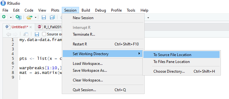
To change via the Session menu, go to Session > Set Working Directory and Choose Directory... if you want to choose a certain directory or have not saved your script file; choose To Source File Location if you have already saved your script on your computer.

The command list.files() produces a character vector of the names of files or directories in the current directory. When you put a path in the parameter, a character vector of the names for the specified directory will be displayed.

setwd("C:/Users/YourNetId/Desktop/RI")
list.files()
 [1] "test.txt"
list.files("C:/Users/YourNetId/Desktop/RI")
 [1] "test.txt"

Data Structures

Vectors

The command c() combines the submitted values into a vector or list.

Usage: P = c(X,Y,Z, ...)

> a = c(1,2,5.3,6,-2,4)
> a
 [1]  1.0  2.0  5.3  6.0 -2.0  4.0
> b = c("male", "female")
> b
 [1] "male"   "female"

Matrices

The command matrix() creates a matrix from a given set of values.

Usage: matrix(data = NA, nrow = 1, ncol = 1, byrow = FALSE, dimnames = NULL)

> a1 = c(1,2,3,4,5,6)
> mat1 = matrix(a1, nrow=2, ncol=3, 
+               dimnames=list(c("R1","R2"),
+               c("C1","C2","C3")))
> mat1
   C1 C2 C3
R1  1  3  5
R2  2  4  6

Data Frames

Data frames are also similar to matrices, but different columns can have different data types (numeric, character, etc.).

Data frames are used as the fundamental data structure by most of R’s modeling software.

Usage: mydata = data.frame(X,Y,Z...)

> a1 = c(1,2,3,4,5,6)
> a2 = c("a","b","c","d","e","f")
> DataFrame = data.frame(a1,a2)
> DataFrame
  a1 a2
1  1  a
2  2  b
3  3  c
4  4  d
5  5  e
6  6  f

Lists

A list is a generic vector containing different objects. The objects in a list can be different types and dimensions.

Usage: myList = list(name=" ", X, Y, Z...)

> a1 = c(2, 3, 5)
> a2 = c("aa", "bb", "cc", "dd", "ee")
> a3 = 15
> myList = list("mylist", a1, a2, a3)
> myList
[[1]]
[1] "mylist"

[[2]]
[1] 2 3 5

[[3]]
[1] "aa" "bb" "cc" "dd" "ee"

[[4]]
[1] 15

Factors

Factors are used to encode a numeric vector into a categorical or ordinal variable.

Usage: myFactor = factor(data)

> a1 = c(1, 2, 1, 2, 1, 3, 3)
> myFactor = factor(a1)
> myFactor
 [1] 1 2 1 2 1 3 3
Levels: 1 2 3

The output displays the factor values.

Importing Data

Importing From a Delimited Text File

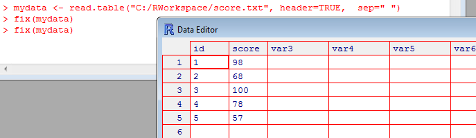
The Data Editor window displays a table.

Importing From a .csv or Text File

The read.csv() command reads a .csv file and sets it as the data object.

Example:

 gssdata = read.csv("R_Data.csv", header=TRUE, 
 na.strings = c("", "NA"), stringsAsFactors = FALSE)

The read.csv() function includes parameters to treat empty strings and “NA” as missing values, and prevents automatic conversion of strings to factors.

In read.csv(), header=TRUE lets R know that the first row of the file is a header with column names.

If the first row does not contain column names, you would use header=FALSE instead.

na.string=c("", "NA") tells the function that both the empty strings or the NA string should be treated as missing (NA).

Because we already set our working directory, we do not need to specify the full (absolute) path to the file, just the file name. If the file is in the working directory, it will be imported.

The stringsAsFactors = FALSE argument is often used in functions like read.csv(), and read.table() to prevent character strings from being automatically converted to factors in R.

Similarly, read.table() can be used to import .txt files. The arguments for this function are very similar to read.csv() except that header is FALSE by default (it is TRUE by default in read.csv).

Data can be viewed by clicking on the name of the data frame in the Environment tab of the Workspace pane.

Importing From an Excel File

Several packages make importing Excel files very easy in R. The two most popular packages are readxl and xlsx. The functions in these packages have similar arguments to other base import functions. Excel import functions will let you specify which sheet to import as well as specific data ranges if your data are not ‘’tidy’’.

    library(readxl)
    xldata = read_excel("my_excel_data.xlsx", range = "C1:E7")

Importing From Another Format

R can import data from SPSS, SAS, and STATA formats using similar methods. You may need to import a package such as haven or foreign to import those formats. For more details, please look up R help. Example:

library(haven)
gssdata = read_dta("StataGSSData.dta")

Data Manipulation and Transformation

Viewing Data

This section explains some frequently used commands to view or grab information about the data.

dataObject$variableName: Displays the vector defined by the variableName contained in the dataObject. Also used to specify a variable for use in other functions.

Example:

gssdata$educ
   [1] 14 10 16 16 18 16 13 12  8 12 19 14 13 16 12 12 16 16
  [19] 20 18 15 14 14 12 16  8 12  9 12 14 12  8 16 16 10 18
  [37] 20 20 19 12 12 12 12 18 16 12 18 18 17 16 14 12 18 18

names(dataObject): Displays the names of variables contained in the dataObject. Recall that we previously defined gssdata as our data object that refers to the actual data that we are pulling up with read.csv command. Therefore, as shown, the command to list variable names in the data is names(gssdata).

names(gssdata)
 [1] "id"       "age"      "year"     "wrkstat"  "hrs1"    
 [6] "marital"  "degree"   "sphrs1"   "postlife" "sex"     
[11] "SIBS"     "agekdbrn" "othlang"  "born"     "neisafe" 
[16] "hsbio"    "hschem"   "tspac"    "nextgen"  "grass"     

str(dataObject): Compactly displays the data structure of the dataObject. We will use gssdata as an example. Submitting the command str(gssdata), we see that it contains 37 variables (which matches the output from names(gssdata). The variables are numeric, factors (categorical), and integers. Variables can also be strings – characters which do not represent categories.

str(gssdata)
'data.frame':   2348 obs. of  37 variables:
 $ id      : int  1 2 3 4 5 6 7 8 9 10 ...
 $ age     : int  43 74 42 63 71 67 59 43 62 55 ...
 $ year    : int  2018 2018 2018 2018 2018 2018 2018 2018 2018 2018 ...
 $ wrkstat : chr  "temp not working" "retired" "working fulltime" "working fulltime" ...
 $ hrs1    : int  NA NA 40 40 NA NA 35 89 40 40 ...
 $ marital : chr  "never married" "separated" "married" "married" ...
 $ degree  : chr  "junior college" "high school" "bachelor" "bachelor" ...
 

View(dataObject) Opens dataObject in the Script pane. Can also be accessed by clicking on the name of the object in the Environment tab of the Workspace pane.

fix(dataObject): Launches the Data Editor and opens dataObject.

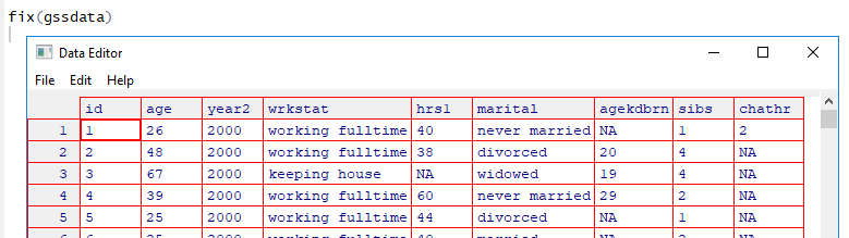
In the Data Editor, you can browse the spreadsheet by scrolling up/down or using the arrow keys. You can also edit data. For example, you might want to change the value of the seventh case of the education variable, educ. To do this, you would move the cursor to the appropriate cell and double-click.

If you need to change a variable name and/or its associated data type, just click the variable of interest on top of the spreadsheet and you will get the variable editor dialog box as follows.

NOTE: Changes you make in the Data Editor will not be saved to your data file! To save these changes, you will need to use write.csv() or a similar function.

attach(dataObject)/ detach(dataObject): Attaches/Detaches a set of R objects to a search path. When a database is attached to the R search path, it means that the database is searched by R when evaluating a variable, so objects in the database can be accessed by simply giving their names. If a database has not been attached, then the variables it contains must be accessed using the $ notation.

Other Useful Functions For Working with Imported Data

dim(object) – Displays dimensions of an object.

dim(gssdata)
[1] 2348   37

head(object) – Get the first several lines of an object.

head(gssdata)
  id age year          wrkstat hrs1       marital
1  1  43 2018 temp not working   NA never married
2  2  74 2018          retired   NA     separated
3  3  42 2018 working fulltime   40       married
4  4  63 2018 working fulltime   40       married
5  5  71 2018          retired   NA      divorced
6  6  67 2018          retired   NA       widowed

tail(object) – Get the last several lines of an object.

tail(gssdata)
       id age year          wrkstat hrs1       marital
2343 2343  19 2018           school   NA never married
2344 2344  37 2018 working fulltime   36      divorced
2345 2345  75 2018 working parttime   36       married
2346 2346  67 2018          retired   NA       married
2347 2347  72 2018          retired   NA       married
2348 2348  79 2018    keeping house   NA       widowed

Descriptive Statistics

In this section, we will introduce several basic statements in descriptive statistics. In the R environment, many packages are not loaded into the console by default and need to be loaded by using the Library() statement.

For instance, you can get concise statistical description of the data using the describe function in the psych package. However, the psych package is not loaded by default. As previously explained (see the “Packages and Library” sub-section in this workbook), it means that you first need to install and load the psych package before you can use any of the functions included in the package.

Summary statistics

The describe() function provides a concise statistical summary for numeric variables. The statistical summary typically includes the number of observations, central tendency statistics (mean, median, sd), range, and skew and kurtosis. The following is the output for the variable age:

> library(psych)
> describe(gssdata$age)
   vars    n  mean    sd median trimmed   mad min max range skew
X1    1 2341 48.97 18.06     48    48.4 22.24  18  89    71 0.22
   kurtosis   se
X1    -0.91 0.37

Exercise 1

Run frequencies for the variable SIBS (number of siblings). 1. What is the total number of cases? 2. What are the mean, median, range and standard deviation of this variable?

Frequencies

Categorical (factor) variables can be summarized in R using frequency and proportion tables. The freq() function prints a frequency table of the selected object. This method is in the descr package, which you may need to install. A bar chart associated with the frequency table will also pop up.

> library(descr)
> freq(gssdata$sex)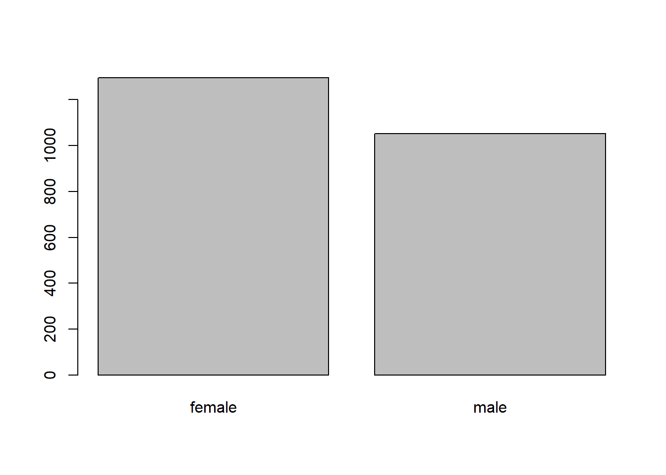
gssdata$sex 
       Frequency Percent
female      1296    55.2
male        1052    44.8
Total       2348   100.0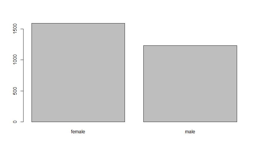

If there are missing values in the variable, freq() will count those and additionally display a Valid Percent that ignores NA values. You can also count NA values using sum(is.na()) (example below).

> freq(gssdata$nextgen)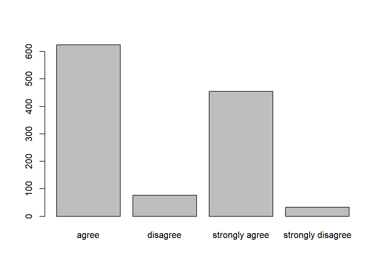
gssdata$nextgen 
                  Frequency Percent Valid Percent
agree                   624  26.576        52.525
disagree                 76   3.237         6.397
strongly agree          455  19.378        38.300
strongly disagree        33   1.405         2.778
NA's                   1160  49.404              
Total                  2348 100.000       100.000
> sum(is.na(gssdata$nextgen))
[1] 1160

Data Transformation

Creating New Variables

To create new variables based on existing variables, use the assignment operator <- or =. Note that to create a new variable in a dataframe, you have to use the object name and $ notation to specify the name of the created variable. For instance, you need to type gssdata$sqrtage rather than sqrtage so that the system understands the newly created variable is an element of gssdata rather than a stand-alone variable.

> gssdata$sqrtage = sqrt(gssdata$age)
> gssdata$age[1:10]
 [1] 43 74 42 63 71 67 59 43 62 55
> sqrtage
Error: object 'sqrtage' not found
> gssdata$sqrtage[1:10]
 [1] 6.557439 8.602325 6.480741 7.937254 8.426150
 [6] 8.185353 7.681146 6.557439 7.874008 7.416198

The above codes create a new variable sqrtage by calculating the square root of the existing age variable.

Tip

Newly created variables are not included in any previous attach() calls. In this example, an error results since variable did not exist when we attached gssdata.

Recoding Variables

The recode procedure transforms an existing variable into a new variable by changing, rearranging, or consolidating the values of the existing variable. It allows the user to:

• Change an existing categorical variable into a new categorical variable with a fewer number of categories/levels.

• Change an existing continuous variable with many unique values (for example, income, age) into a categorical variable with few levels (for example, variable incomeRecode will have low, medium, and high as values, ageRecode will have young, adult, senior as values).

• Code missing values.

• Replace miscoded values with correct values.

• Create a dummy variable upon a cutoff value.

To recode a variable, one or more of R’s logical operators are used. The following table lists R’s common logical operators.

Operator	Description
==	Equal to
!=	Not equal to
<	Less than
>	Greater than
<=	Less than or equal to
>=	Greater than or equal to
!x	Not x
x	y
x & y	x AND y
isTRUE(x)	Test if x is TRUE

Note: x and y are expressions.

The basic syntax is:

newVariable[ConditionOnExistingVariable] = newValue

The newValue part of the syntax will only execute when the specified ConditionOnExistingVariable is TRUE.

For instance, you can transform a continuous variable, such as age, into a categorical variable. In this example, the new variable is called agecat and has three levels: young, middle aged, and elder.

> gssdata$agecat[gssdata$age > 75] = "Elder"
> gssdata$agecat[gssdata$age > 45 & gssdata$age <= 75]="Middle Aged"
> gssdata$agecat[gssdata$age <= 45] = "Young"
> gssdata$agecat[1:10]
 [1] "Young"       "Middle Aged" "Young"      
 [4] "Middle Aged" "Middle Aged" "Middle Aged"
 [7] "Middle Aged" "Young"       "Middle Aged"
[10] "Middle Aged"   
 > class(gssdata$agecat)
 [1] "character"

We can see this new variable in the Data Editor,

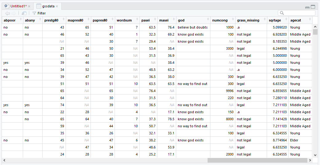
You may want your data to be structured as a factor variable rather than a character/string variable. This can be accomplished by declaring the data to be factors, and identifying the levels with the factor() function.

> gssdata$agecat2 = factor(gssdata$agecat, 
 levels=c("Young","Middle Aged","Elder"))
> head(gssdata$agecat2)
[1] Young       Middle Aged Young       Middle Aged
[5] Middle Aged Middle Aged
Levels: Young Middle Aged Elder
> class(gssdata$agecat2)
[1] "factor"

You will see that R shows the first six values of agecat2 and has recognized it as a factor. head() also shows the three levels in agecat2: Elder, Middle Aged, and Young. You can double how R recognizes agecat2 by using the str() or levels() functions.

> str(gssdata$agecat2)
  Factor w/ 3 levels "Young","Middle Aged",..: 1 2 1 2 2 2 2 1 2 2 ...
> levels(gssdata$agecat2)
[1] "Young" "Middle Aged" "Elder"

Lastly, to verify that the variable has been recoded correctly, simply run a frequency on both the original variable and the recoded variable using the table() command.

> table(gssdata$agecat2, useNA="ifany")

      Young  Middle Aged   Elder   <NA> 
       1077         1079     185      7 

Here, in the recoded variable agecat, the elder group includes 185 people, the middle aged group includes 1079 people and the young group has 1077.

We can also use the command subset() to get all the people in the elder group and use dim() to count the number of people in this group. By repeating this procedure for the rest of the groups we see that there are 185 people classified as elder, 1079 people classified as middle-aged, and 1077 people classified as young. From this, we can conclude our recoding is correct.

> elderdata = subset(gssdata, gssdata$age>75)
> dim(elderdata)
[1] 185  40
> middleAgeddata = subset(gssdata, (gssdata$age > 45 
 & gssdata$age <= 75) )
> dim(middleAgeddata)
[1] 1079   40
> youngdata = subset(gssdata, gssdata$age <= 45)
> dim(youngdata)
[1] 1077   40

Exercise 2

Create new variables to represent the recodes of the variable hrs1 (number of hours worked in the last week) into less than 40 and more than 40 (two groups), and recode all missing values to NA. Be sure to check the new variables by creating a frequency table.

Multivariate Tables

table()

The table() function creates a contingency table. A contingency table is used to show the joint distribution of cases over two or more categorical variables. The basic syntax to produce a contingency table, mytab = table(var1, var2), will result in a table with var1 in the rows and** var2** in the columns. Let’s create a contingency table using the variables postlife and sex. In our dataset, postlife contains information telling us if the respondent believes in life after death, and sex is the gender of the respondent.

> table(gssdata$sex, gssdata$postlife)
        
          no yes
  female 161 1017
  male   242 703
> table(gssdata$sex, gssdata$postlife, useNA="ifany")
        
           no  yes <NA>
  female  161 1017  118
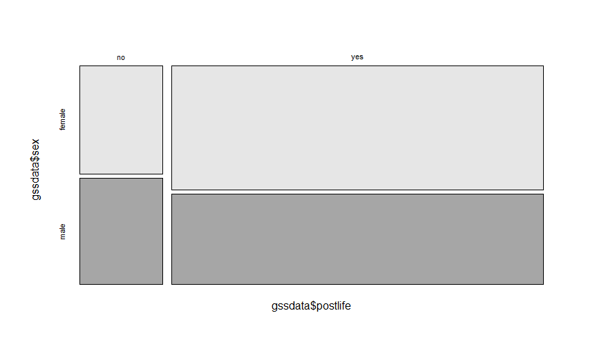
  male    242  703  107

crosstab() or CrossTable()

The crosstab(), or CrossTable(), function creates a crosstab, which allows you to compare two or more categorical variables. The crosstab command is easier to use and more sophisticated than the base R table() command. It allows for chi-squared tests and other more specialized outputs. In order to use this command, you must first install the library descr. Once installed, establish it as the package in use: library(descr). Again, to learn about the commands within this library you can enter library(help=descr). Now we will reproduce our contingency table comparing postlife and sex using the crosstab() function.

> crosstab(gssdata$sex, gssdata$postlife)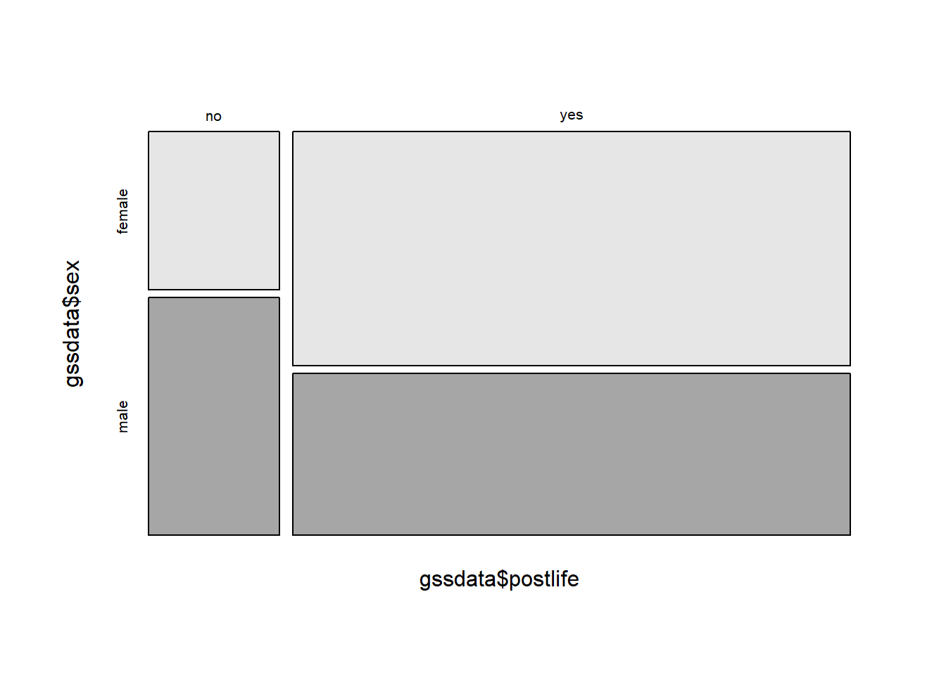
   Cell Contents 
|-------------------------|
|                   Count | 
|-------------------------|

=================================
                gssdata$postlife
gssdata$sex     no    yes   Total
---------------------------------
female         161    1017    1178
---------------------------------
male           242    703     945
---------------------------------
Total          403   1720    2123
=================================

To get row, column, and/or total percentages, add prop.r=TRUE, prop.c=TRUE, and/or prop.t=TRUE to the function like so:

> # column percentage
> crosstab(gssdata$sex, gssdata$postlife,prop.c = TRUE)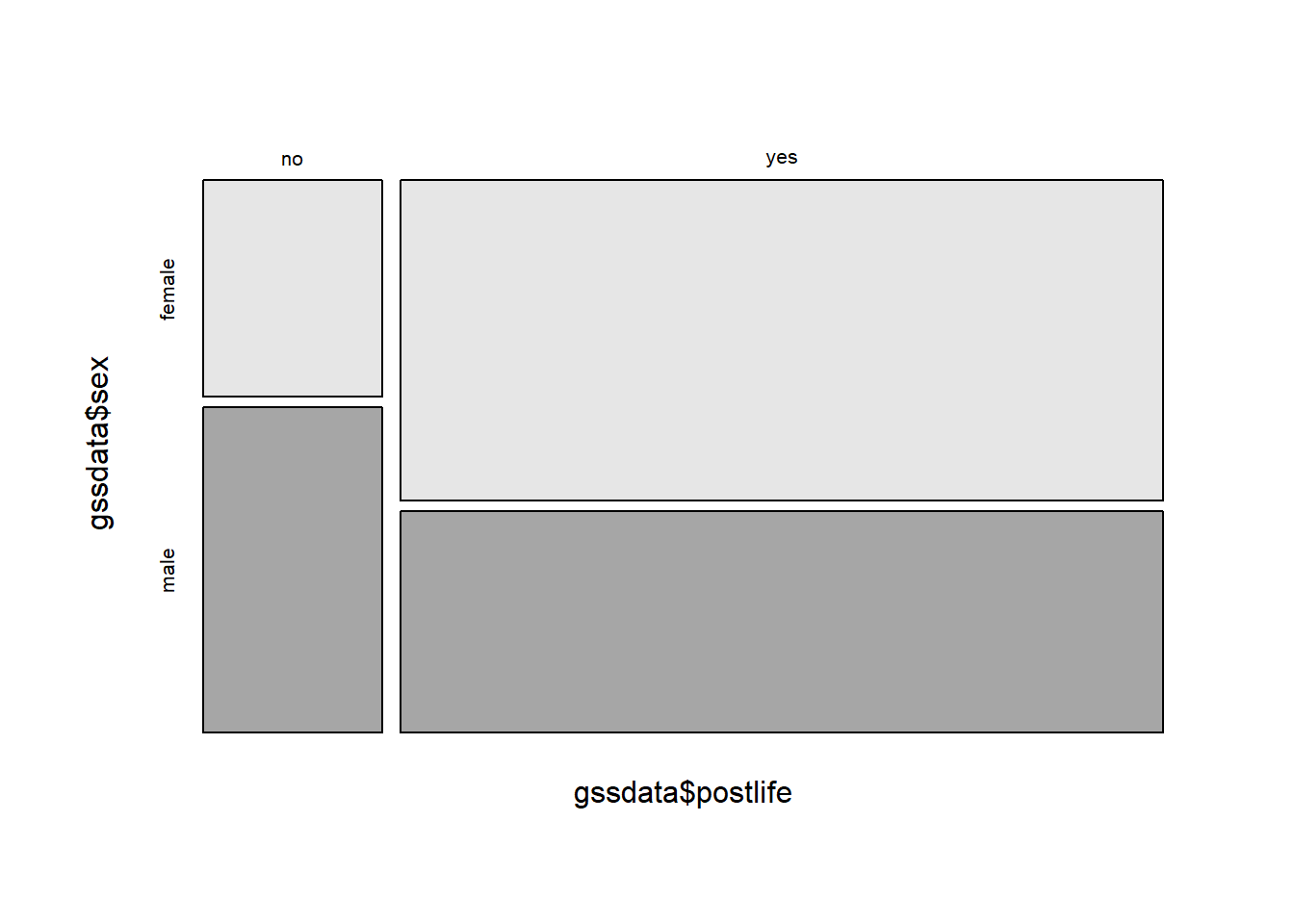
   Cell Contents 
|-------------------------|
|                   Count |
|           Column Percent| 
|-------------------------|

====================================
               gssdata$postlife
gssdata$sex       no     yes   Total
------------------------------------
female          161    1017    1178 
               40.0%   59.1%        
------------------------------------
male            242     703     945 
               60.0%   40.9%        
------------------------------------
Total           403    1720    2123 
                 19%     81%        
====================================

Exercise 3

Find out how many foreign-born and native-born survey respondents can speak a language other than English. That is, run a crosstab using variables othlang (Can respondent speak a language other than English?) and born (Was respondent born in this country?).

Graphics

Histogram

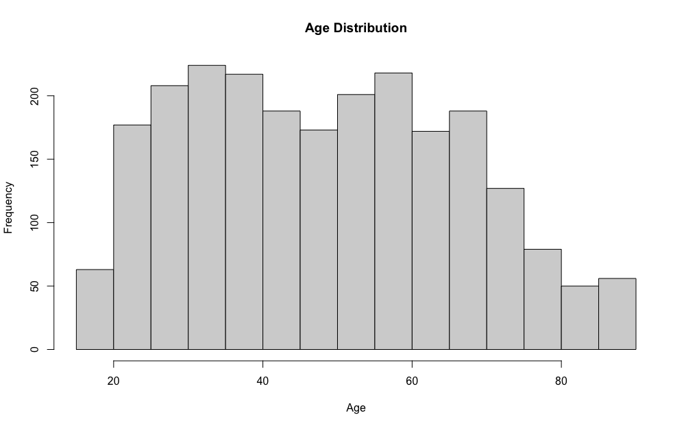
A histogram visually displays the distribution of a continuous variable. In R, the hist() command works as shown below:

hist(gssdata$age, main='Age Distribution', xlab='Age')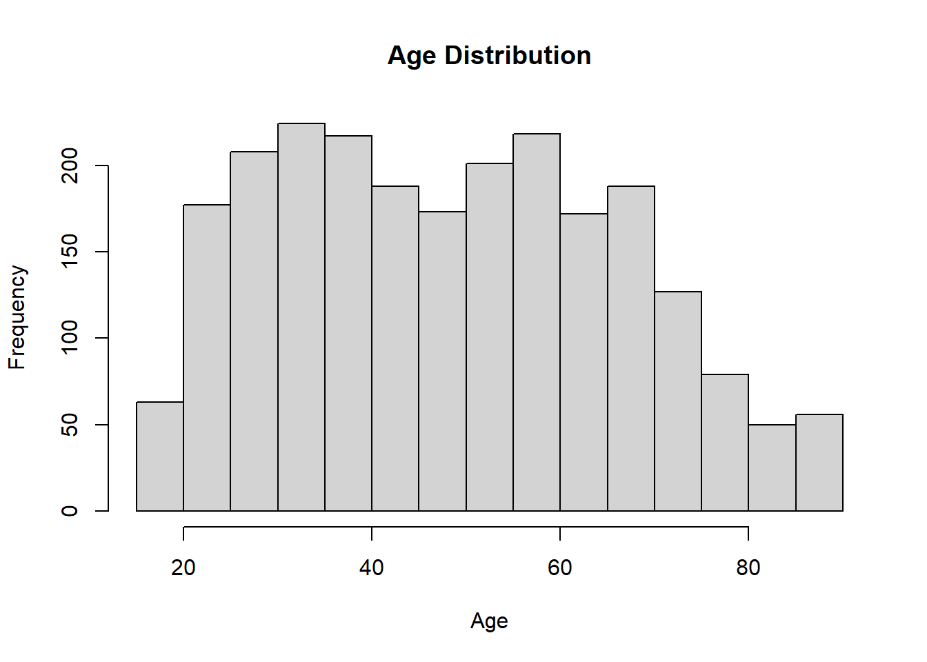

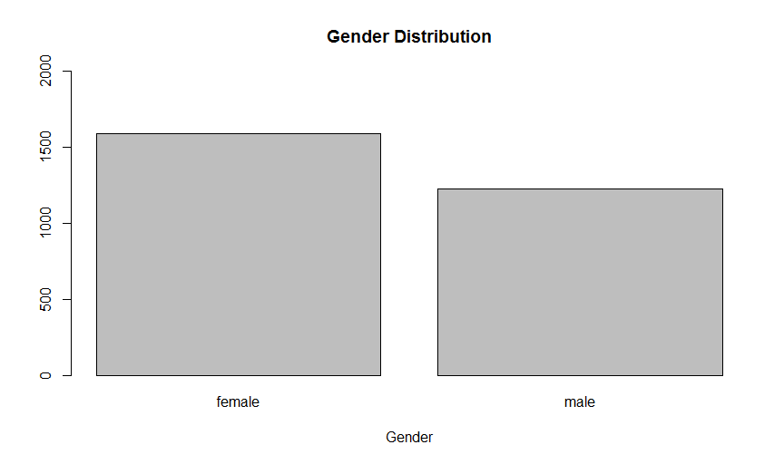
Bar Graph

A bar graph can display the frequencies or distribution of a categorical variable. First, a data table must be created for plotting. In this case, we named our data table counts:

> countSex = table(gssdata$sex)
> barplot(countSex, main="Gender Distribution",
 xlab="Gender", ylim=c(0, 2000))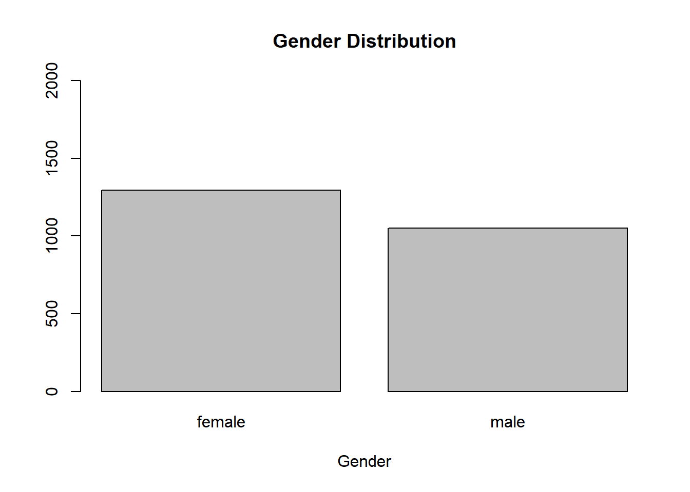

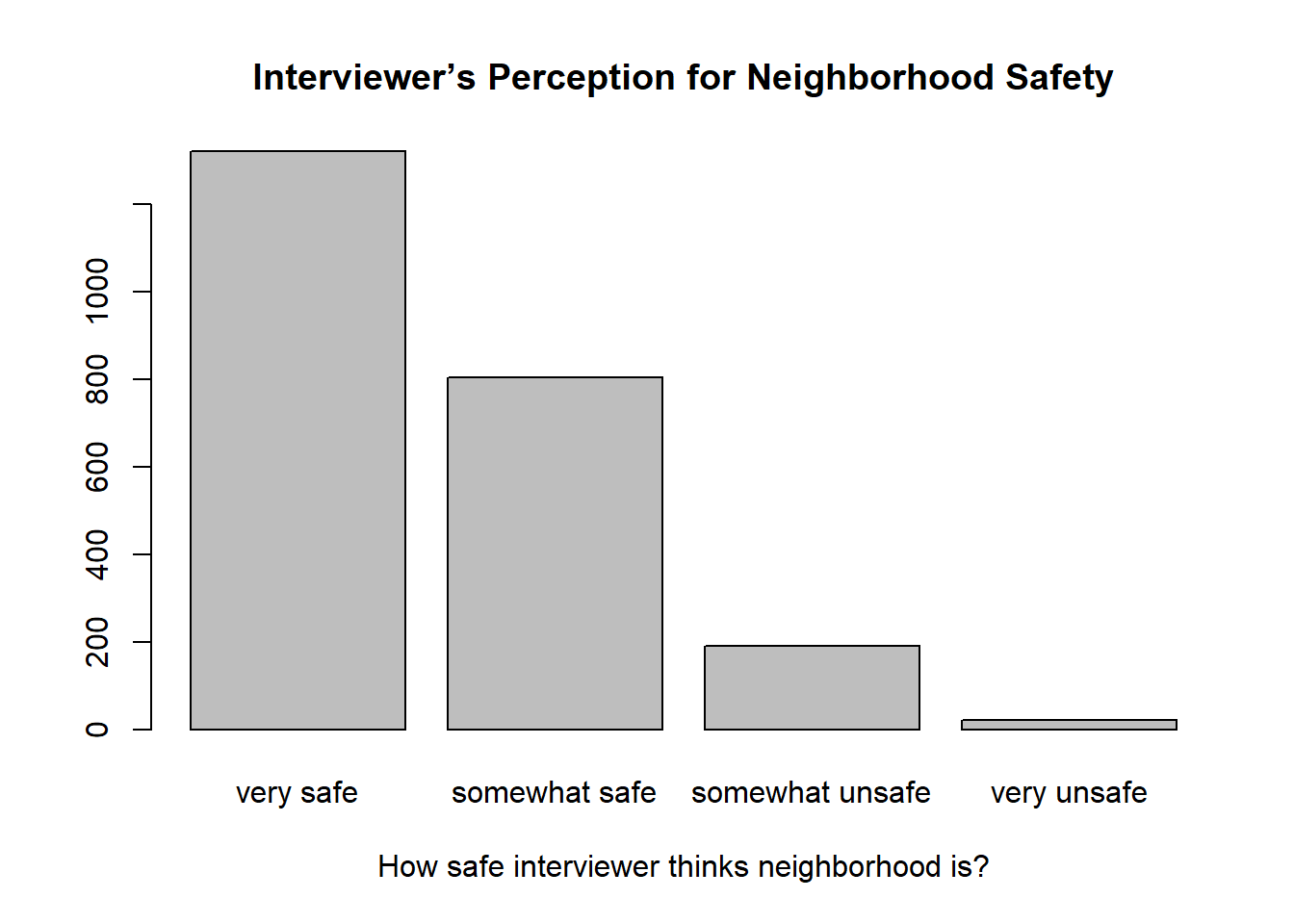
Exercise 4

Create a bar chart for the variable neisafe. This variable is based on the question, “How safe interviewer thinks neighborhood is?” . The answers are categorized as: very safe, somewhat safe, somewhat unsafe, very unsafe. Include the title “Interviewer’s Perception for Neighborhood Safety”.

Grouped Bar Graph

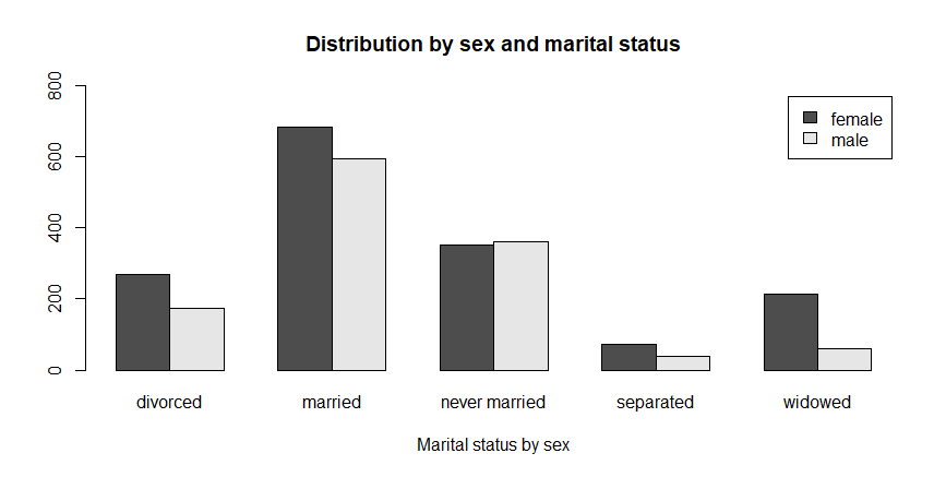
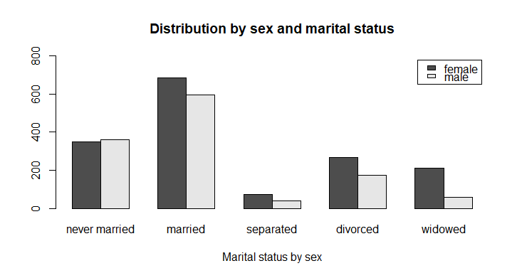
A grouped bar graph is a bar graph that uses an additional variable to group the plotted data.For example, create a grouped bar graph displaying sex and marital. First, a data table must be created for plotting. In this case, we named our data table counts:

counts = table(gssdata$sex, gssdata$marital)

Next, add the syntax for the bar plot, where main is the title for the graph, xlab is the x-axis label, and ylim is used to set the y-axis height, in this case 600.

> counts = table(gssdata$sex, gssdata$marital)
> barplot(counts, 
         main= 'Distribution by sex and marital status',
         xlab = 'Marital status by sex',
         ylim = c(0,800),
         legend = rownames(counts), beside = TRUE)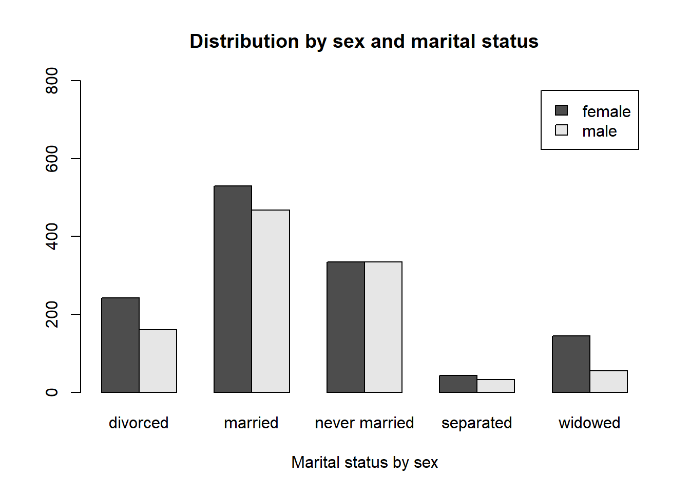

To reorder the marital status categories, try the following syntax. Another great package for plotting is called ggplot2. ggplot2 is extremely customizable and produces beautiful plots. We will produce this plot using ggplot2 code:

> # reorder categories
> table(gssdata$marital)

     divorced       married never married     separated 
          403           998           670            75 
      widowed 
          200 
> 
> gssdata$marital2 = factor(gssdata$marital,c("never married","married",
   "separated","divorced","widowed"))
> 
> #ggplot2 way
> library(ggplot2)
> ggplot(data=subset(gssdata,!is.na(gssdata$marital2)), 
        aes(marital2,fill=sex)) 
   geom_bar(position="dodge") 
   scale_fill_grey() 
   xlab("Marital Status by Sex") 
   theme_minimal()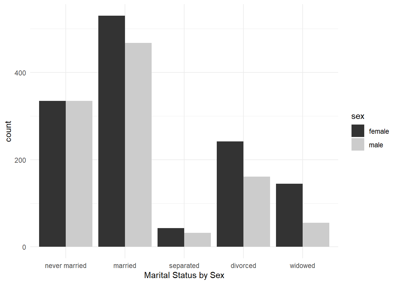

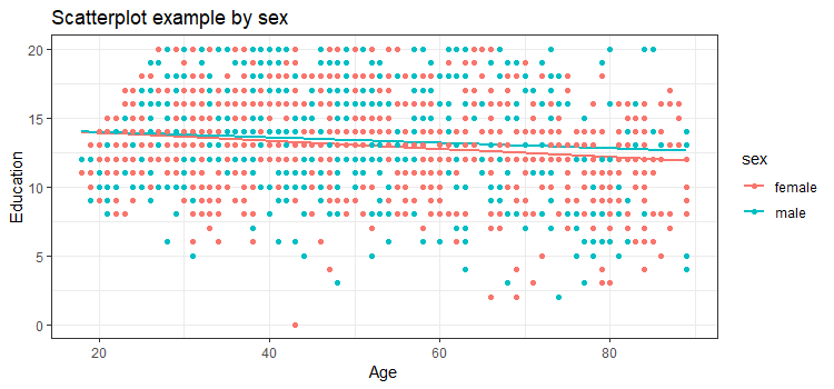
Scatterplot

A scatterplot plots the “positions” of two variables in dimensions x and y. We run the plot() function:

plot(gssdata$age, gssdata$educ,  main="Scatterplot Example", 
 xlab="Age", ylab="Education")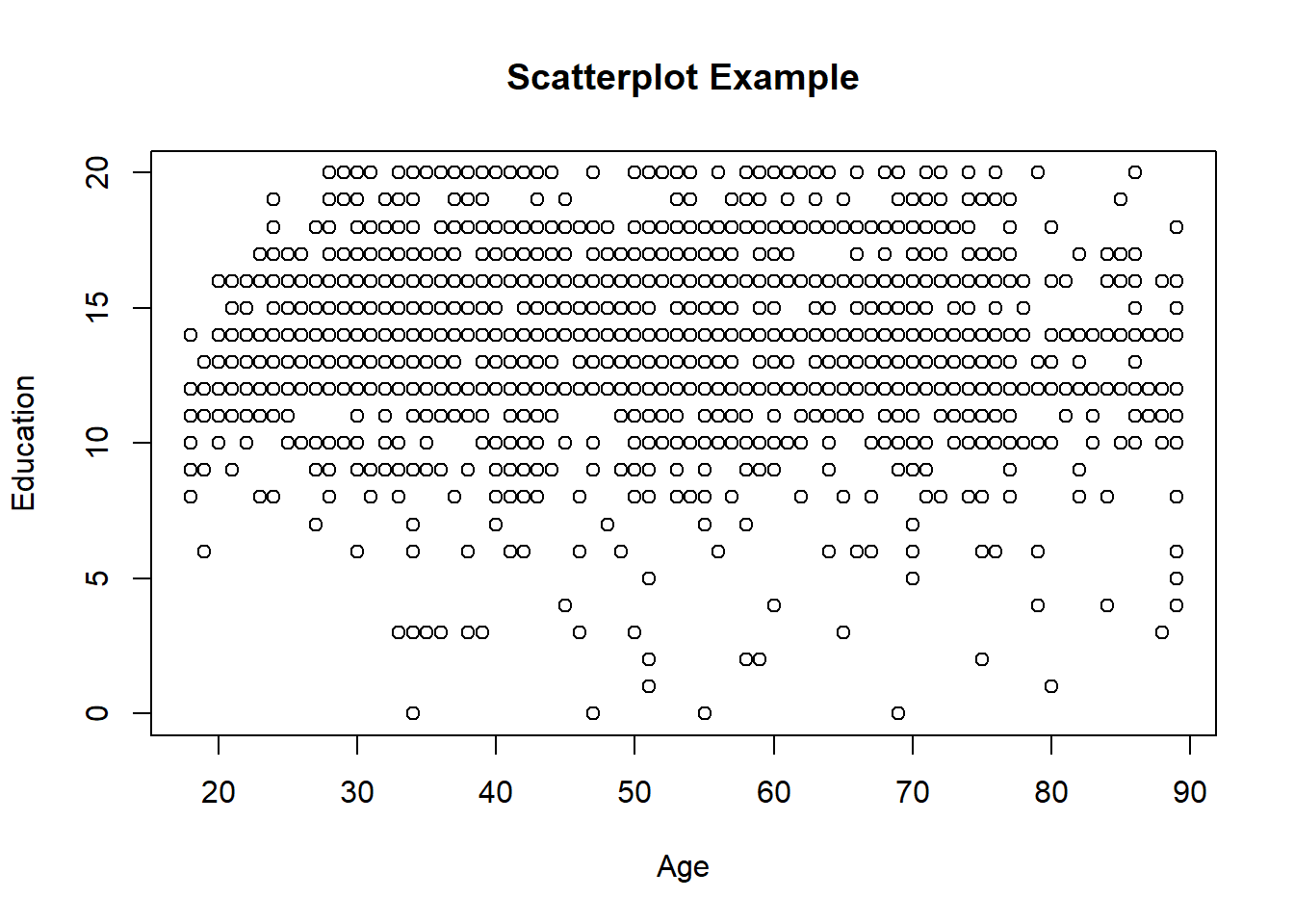

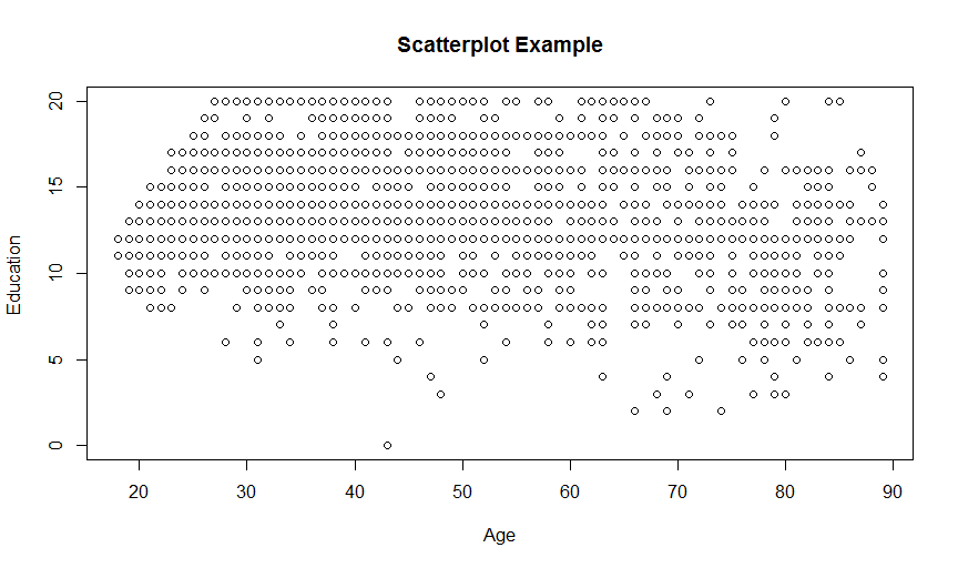
Here’s the plot using ggplot2, filling the points and fitting linear regression lines by sex:

    > library(ggplot2)
    > ggplot(gssdata, aes(x = age, y = educ, color = sex)) +
  geom_point() +
  geom_smooth(method = "lm", se = FALSE) +
  xlab("Age") +
  ylab("Education") +
  ggtitle("Scatterplot Example by Sex") +
  theme_bw()
    Warning messages:
1: Removed 10 rows containing non-finite outside the scale range (`stat_smooth()`). 
2: Removed 10 rows containing missing values or values outside the scale range (`geom_point()`).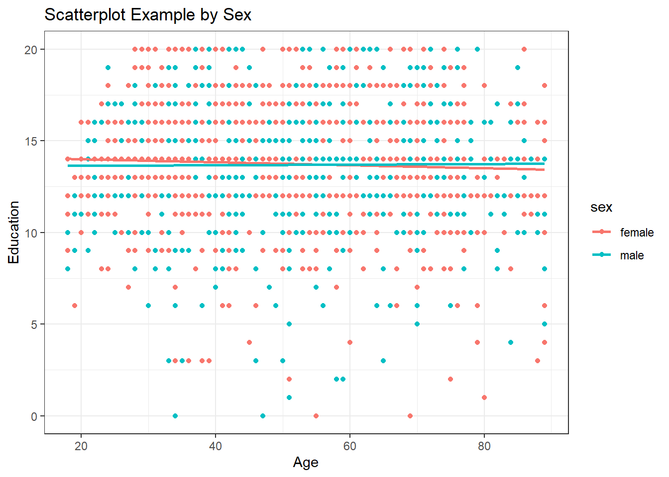  

Note: the warning message just displays how many missing values were removed from the plotted data.

Saving and Printing

Output data can be exported to many different file formats. For example:

write.table(gssdata, file = "SAVE_OUT_Example_GSS.txt",
             append = FALSE, sep = ",")

This statement exports the modified gssdata to a text file using “,” as the separator. If append = TRUE, the gssdata will be appended to the current file.

write.csv(gssdata, file = "SAVE_OUT_Example_GSS.csv", row.names=F)

This statement exports the modified gssdata to a csv file.

Finally, you can save your data out in R format. This is useful to keep all the features of the data that you have worked on – for example, keeping factor orderings. Saving out the data as a text file would not preserve that information.

save(gssdata, file="SAVE_OUT_Example_GSS.RData")

To read these data back into R you use the load() function. Once you do this, you can use ls() to check the names of the objects in your Workspace and use the loaded objects.

load("SAVE_OUT_Example_GSS.RData")

Appendix : Exercises and Answers

R1_script_complete.R

Exercise 1

Run frequencies for the variable sibs (number of siblings). 1.What is the total number of cases? 2.What are the mean, median, range and standard deviation of this variable?

Answer

If you want to calculate the mean, median, range, and sd separately, you can use the following code (removing missing values before computation):

> length(gssdata$SIBS)
[1] 2348
> # without nas:
> sum(!is.na(gssdata$SIBS))
[1] 2343
> mean(gssdata$SIBS, na.rm = TRUE)
[1] 3.579599
> median(gssdata$SIBS, na.rm = TRUE)
[1] 3
> range(gssdata$SIBS, na.rm = TRUE)
[1]  0 25
> sd(gssdata$SIBS, na.rm = TRUE)
[1] 2.863154

You can also get these values at once using the describe function in psych.

> library(psych)
> describe(gssdata$SIBS)
   vars    n mean   sd median trimmed  mad min max
X1    1 2343 3.58 2.86      3    3.17 2.97   0  25
   range skew kurtosis   se
X1    25 1.75     5.36 0.06

Exercise 2

Create a new variable to represent the recodes of the variable hrs1 (number of hours worked in the last week) into less than 40 and more than 40 (two groups), and recode all missing values to NA. Be sure to check the new variable by creating a frequency table.

Answer

We can easily recode this variable by coding the categories as characters and converting them into a factor.

> gssdata$recodeHrs = NA
> gssdata$recodeHrs[gssdata$hrs1 < 40 & gssdata$hrs1 >= 0] = "Less than 40"
> gssdata$recodeHrs[gssdata$hrs1 >= 40] = "More than 40"
> str(gssdata$recodeHrs)
 chr [1:2348] NA NA "More than 40" "More than 40" NA NA "Less than 40" ...
> 
> gssdata$recodeHrs = factor(gssdata$recodeHrs)
>
> str(gssdata$recodeHrs)
Factor w/ 2 levels "Less than 40",..: NA NA 2 2 NA NA 1 2 2 2 ...

Note that we skipped coding the numeric values of this variable, but when we converted it to a factor, R automatically created numeric values for us.

Comparing the the number of observations and NAs in each variable, we can ensure that the variable recode was performed correctly.

> descr(gssdata$recodeHrs)
Less than 40 More than 40         NA's 
         419          962          967 
>
> freq(gssdata$recodeHrs)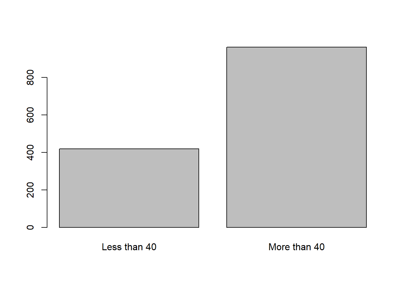
gssdata$recodeHrs 
             Frequency Percent Valid Percent
Less than 40       419   17.84         30.34
More than 40       962   40.97         69.66
NA's               967   41.18              
Total             2348  100.00        100.00 

Exercise 3

Find out how many foreign-born and native-born survey respondents can speak a language other than English. That is, run a crosstab using variables othlang (Can respondent speak a language other than English?) and born (Was respondent born in this country?).

Answer

> crosstab(gssdata$othlang, gssdata$born, prop.c=TRUE)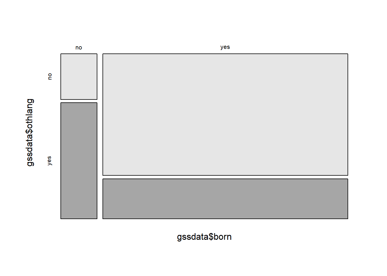
   Cell Contents 
|-------------------------|
|                   Count | 
|          Column Percent | 
|-------------------------|

========================================
                   gssdata$born
gssdata$othlang       no     yes   Total
----------------------------------------
no                   85    1537    1622 
                   28.1%   75.2%        
----------------------------------------
yes                 217     506     723 
                   71.9%   24.8%        
----------------------------------------
Total               302    2043    2345 
                   12.9%   87.1%        
========================================

Exercise 4

Create a bar chart for the variable neisafe. This variable is based on the question, “How safe interviewer thinks neighborhood is?” . The answers are categorized as: very safe, somewhat safe, somewhat unsafe, very unsafe. Include the title “Interviewer’s Perception for Neighborhood Safety”.

Answer

> neisafe_table = table(gssdata$neisafe)
> neisafe_table

somewhat safe somewhat unsafe       very safe     very unsafe 
            805             191            1322              22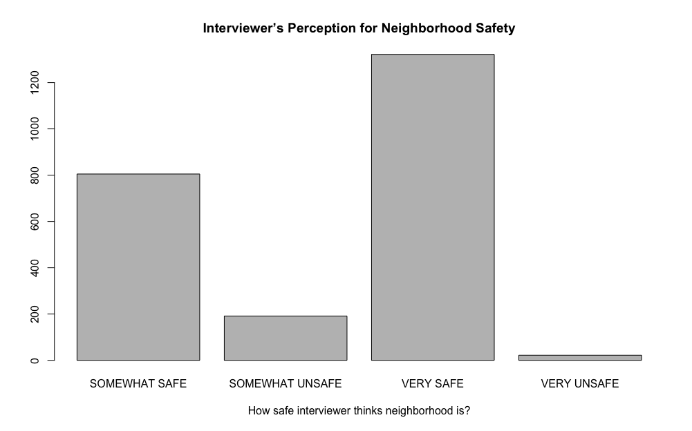 

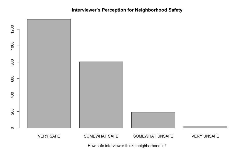
To draw the bar chart for a variable in the data frame, we can create a table object, which can be used as the first parameter in the barplot() function. The main and xlab arguments of this function are used to display the main title and the x-axis title, respectively.

To reorder the categories we use the factor() function.

First look at the levels:

> gssdata$neisafe <- factor(gssdata$neisafe)
> levels(gssdata$neisafe)
[1]   "somewhat safe"  "somewhat unsafe"   "very safe"   "very unsafe" 

> table(gssdata$neisafe)

  somewhat safe     somewhat unsafe       very safe  very unsafe 
            805             191            1322          22

## or reordered:
> gssdata$neisafe2 = factor(gssdata$neisafe,
                            c("very safe", "somewhat safe",
                            "somewhat unsafe","very unsafe"))

> neisafe_table_ordered<-table(gssdata$neisafe2)
> neisafe_table_ordered

very safe  somewhat safe  somewhat unsafe   very unsafe
    1322             805             191              22 
    
    
> barplot(neisafe_table_ordered, 
main = "Interviewer’s Perception for Neighborhood Safety",
xlab = "How safe interviewer thinks neighborhood is?")