SAS I
Getting Started with SAS
After attending this training session, you should understand the following:
- The elements of the SAS environment under Windows
- The general structure of SAS programming syntax
- How to submit SAS programs
- How to use and save SAS data files
- How to create, delete, recode, and otherwise manipulate variables
- Options to control the formatting of output
- How to include helpful comments in your output
- How to save your output to text or generic HTML files
- How to create charts
- How to save SAS programs
- How to print from SAS
- Where to go for additional help
Introduction
Code and Dataset
For this training session, please download the following data and code:
What is SAS?
SAS is a software package for the management and analysis of data. SAS is not a menu or command driven program. SAS users write a series of instructions called a SAS program using statements referred to as SAS language. While this can initially require a steeper learning curve than other statistical programs, learning SAS will give you access to one of the most powerful statistical software packages available and give you a skill many employers look for. SAS is available to via Illinois AnyWare:. Illinois AnyWare is available to University of Illinois, Urbana-Champaign students at any time and to instructors for academic purposes. SAS also created a university edition of SAS, called SAS OnDemand for Academics, that is free for educational and training purposes. This program runs through a virtual machine and also has tutorials available as well.
To find out more about jobs requiring SAS programming experience, visit http://www.sasjobs.com.
SAS Programs
When we use SAS, we write a series of statements that, when taken together, create a SAS program. The program communicates what you want to do and is written in the SAS language. Because a SAS program is a sequence of statements executed in order, the statements must be appropriately placed in the program.
Writing SAS Programs
When writing SAS statements and programs:
- SAS statements are not case-sensitive.
- SAS statements may continue over multiple lines.
- SAS statements may appear on the same line as other statements.
- SAS statements can start in any column.
- All SAS statements must end with a semicolon;
- SAS programs typically end with a run; statement while some procedures also require a quit; statement to end.
If an error is made in writing a statement, a message will appear in red font in the Log. The log may also contain warnings which appear in green. Warnings indicate that SAS found an issue that may affect the results, but that did not prevent the program from running.
Two Parts of a SAS Program
SAS programs are constructed from two basic building blocks: Data steps and Proc steps.
A typical program begins with a Data step, which creates a SAS data set for analysis or manipulation. Data can be read from files previously created in SAS, data that is manually entered, or from files created by another program (e.g., MS Excel, SPSS). Variables can be created or transformed and datasets can be combined in the data step.
The Proc step, which stands for procedure, is used to perform a statistical, graphing, or other kind of procedure with the data defined in the data step.
A SAS step ends when it encounters a run statement or a new data or proc step.
Starting SAS
To launch SAS, click on the Start button. Navigate to and click the SAS folder, then click SAS 9.4.
The SAS Environment
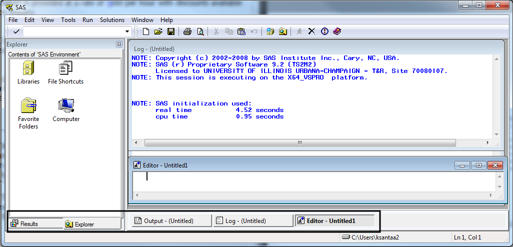
The SAS environment is composed of six main windows. Each window is accessible from a tab near the bottom of the windows. Reading from left to right across the screen they are:
- Results: A Table of Contents for the Results Viewer window, which lists each part of the output in an outline form.
- Explorer: Provides access to SAS files and libraries.
- Output: This tab is typically not used in SAS 9.4 and will remain blank.
- Log: Displays any notes, errors, or warnings about a program, as well as the program statements themselves, after a SAS program has been submitted.
- Editor: Used to type in, edit, and submit SAS programs. In the Windows operating system, the default editor is the Enhanced Editor which is syntax sensitive and color codes your programs making it easier to read and find mistakes.
- Results Viewer: Displays outputs from SAS procedures. This tab is not available until results are generated.
SAS Libraries
In SAS, files including data is stored and accessed through libraries. A SAS library is a group of files that are stored in the same file or directory. Existing SAS Libraries can be found in the Explorer window and several libraries are automatically created at the start of each SAS Session. To create your own library to access your data: 1. Save your data file to a folder on your computer. 2. In SAS, navigate to the Explorer window. 3. In the Explorer, right click and select New. A dialogue box for New Library will open. 4. Enter your library name. Library names in SAS can be up to 8 characters, can only contain alphanumeric characters and underscores (_), and must start with a letter or underscore. 5. Enter the file path for your folder or use Browse… to navigate to the folder location. 6. If you want this library to be created every time you start SAS check the box next to “Enable at startup”. 7. Click “Ok” to create the library.
Save the gss2000sasi.sas7bdat file to your computer. Create a library called “training” that references where this file is saved. We will use this library throughout the workbook.
Temporary and Permanent Datasets
SAS has both temporary and permanent datasets. A permanent dataset is one that will be saved when you close your SAS session while a temporary dataset is is erased when you exit the SAS session. To create or reference a permanent dataset you must use a two part name: libname.dataset where libname is your library name and dataset is the dataset name. Only referencing the dataset name will create a temporary dataset that can be found in the SAS Work library. All files in the Work library are erased when you exit the SAS session and a permanent dataset must be created to save any datasets for future use.
Opening a Data Set
The SAS program below creates a temporary dataset using GSS 2018 data that you have saved into the training library. A line by line explanation of the code is listed below.
data newgss2018;
      set training.gss2018sasi;
      YearBorn = 2018 - age;
run;- Specifies the name for the new dataset which will be created in the
Worklibrary. Dataset names may be up to 32 characters in length and may begin with either a letter or an underscore ( _ ). Special characters (i.e., *, & , ## ) and spaces must not be used in SAS dataset names. - Identifies the name and location of an existing dataset that is to be read into the new dataset.
- Identifies a new variable to be created in the new dataset, YearBorn, which is calculated by subtracting the variable age from 2018 (the year of data collection).
- Closes the SAS data step.
Executing a SAS Program
Once you write a SAS program, you must submit it in order for it to be executed. To submit the program, highlight the portion of the program you want to run in the Editor and click the Submit icon in the toolbar at the top of the screen.
Stopping a SAS Program
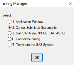
After a SAS program has been successfully executed, SAS will stop and await further instructions.
Sometimes, you may wish to stop execution of a program before it is complete (e.g., for extremely large data sets or infinite loops). To cancel execution of the program, click the Break icon in the toolbar. In the Tasking Manager dialog box that appears, select the Cancel Submitted Statements and press OK.
Exercise 1
- Run the data step below to create a temporary dataset for use in this workshop, newgss2000. After submitting the program, navigate to the Work library in the Explorer window to verify that the new dataset was created.
- Make sure to observe what happens in the various windows of SAS when submitting this program. (See Appendix A for answers.)
data newgss2018;
      set training.gss2018sasi;
run;
Working with Data: The SAS Data Step
Dropping Variables
To drop a variable from a dataset, include a drop statement in the data step.
The drop statement prevents the specified variable(s) from being written to the new dataset identified in the data step. Because the variable is not removed from the dataset until the end of the data step, it is available for the computation of new variables in the data step. For example, to drop the variable degree when creating the ourgss2018 dataset:
 data dropgss;
      set newgss2018;
      drop degree;
 run;
You can check the id for variables by selecting its attributes:
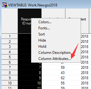
Keeping Variables
The keep statement is used to specify the variable(s) that are to be kept in the new dataset. The variables listed in this statement will be the only variables written to the new dataset. For example, to keep only the variables sex,educ, and realrinc in the ourGSS2018 dataset:
 data keepgss;
      set newgss2018;
      keep sex degree realrinc;
 run;
Creating Variables
Variables are created or redefined in the SAS data step with assignment statements using this basic form: variable = expression.
On the left side of this expression is a variable name, either new or old. The right side of the equation may be a constant, another variable, or a mathematical expression. Here are some examples:
data ourgss2018;
    set newgss2018;
 YearBorn = 2018 - age;
 BirthYear = YearBorn;
 LogIncome = log(realrinc);
 IncomeSquared = realrinc**2;
 totalHourcouple = hrs1 + sphrs1;
      totalHourcouple2 = sum(hrs1, sphrs1);
run;
Line 3 creates a new variable YearBorn by subtracting the respondent’s age (age) from the year the data was collected (2018).
Line 4 creates a new variable BirthYear by copying the values of the variable YearBorn.
Line 5 creates a new variable LogIncome by computing the log of the respondent’s income realrinc.
Line 6 creates a new variable IncomeSquared by squaring the respondent’s income realrinc. Note: To raise a value to a power, two asterisks (**) must be used. If only one asterisk (*) is used, the values will be multiplied.
There are two methods available to sum the values of two or more variables into a single variable. For example, to create a new variable that measures the number of hours spent on the internet:
- In the first statement, the variable is computed by adding the values using the + operator.
- In the second statement, the variable is computed by using the sum expression.
The difference between the two statements lies in their treatment of missing values.
When computing a new variable using an arithmetic operator (e.g. + or -), SAS ignores cases with missing values on any of the component variables. Subsequently, all cases with at least one missing value in either component variable are given a missing value for the newly created variable.
Alternatively, when you use the sum function (i.e. sum(numexpr, numexpr)), SAS calculates a value for a new variable based on all valid values for the component variables. If a case has only one variable with a valid value, only that variable will be used in creating the new variable.
Recoding Variables
Recoding changes, rearranges, or consolidates the values of an existing variable.
If you have a variable with multiple categories, you might want to reduce the number of categories to a more manageable number. For example, a respondent’s employment status (workstatus) has 8 categories, which are listed as follows:
- ft = Working full time
- pt = Working part time
- tn = Temporarily not working
- un = Unemployed, laid off, looking for work
- re = Retired
- sc = In school
- ke = Keeping house
- ot = Other
Variables are recoded in SAS using a series of if…then statements in the data step. The expression takes the form: if expression then statement ; .
To recode employment status (workstatus) from string values into a new variable wrkstat with numeric values:
data a;
      set newgss2018;
      if workstatus = 'ft' then wrkstat = 1;
      if workstatus = 'pt' then wrkstat = 2;
      if workstatus = 'tn' then wrkstat = 3;
      if workstatus = 'un' then wrkstat = 4;
      if workstatus = 're' then wrkstat = 5;
      if workstatus = 'sc' then wrkstat = 6;
      if workstatus = 'ke' then wrkstat = 7;
      if workstatus = 'ot' then wrkstat = 8;
run;
Each statement begins by identifying the string value of the original variable (i.e., if workstatus = \('\)ft\('\)) and then specifies the numeric value of the new variable (i.e., then wrkstat = 1;).
A series of if…then statements may also be used to recode variables to reduce the number of categories in a variable. For example, you can regroup people as “In the labor force” (wrkstat values 1 through 3) and “Not in the labor force” (wrkstat values 5 through 8):
data c;
      set a;
      if 1 <= wrkstat <= 4 then wrkstatRecoded = 1;
      if 5 <= wrkstat <= 8 then wrkstatRecoded = 2;
run;- Line 3 identifies the range of values that are considered ``In the labor force’’ in the if portion of the statement and then specifies the value of the new variable wrkstatRecoded.
- Line 4 identifies the range of values that are considered ``Not in the labor force’’ in the if portion of the statement and then specifies the value of the new variable wrkstatRecoded.
Note: You can specify and apply value labels to future outputs using proc format as described in Section 8.1.
Exercise 2
In the newgss2018 dataset recode the variable degree to create a new variable bachelor_degree that identifies respondents with at least a Bachelor’s degree. Note: that in the provided data degree variable is categorized as follows: 0= Less than High School, 1= High School, 2= Junior College, 3= Bachelor, 4= Graduate (See Appendix A for answers.)
Running Procedures - The SAS Proc Step
Once data is made available for analysis in a data step, a procedure can be run on it. All SAS procedures have required statements and many have optional statements. All procedures start with the keyword proc, followed by the name of the procedure (e.g., proc print or proc contents).
While proc steps often follow a data step, a data step is not needed to execute a procedure on an existing SAS data file if the variables do not require transformation.
Printing & Summarizing Data
Proc Contents
The contents procedure provides a description of a SAS dataset. For example, to view the description of the ourgss2018 dataset, run the following:
proc contents data = ourgss2018;
run;
It will show the general information about this data set.
Some useful options that can be included in the proc contents statement:
- short - outputs a list of variable names
- varnum - lists variables by their position number in the dataset rather than alphabetically
- fmtlen - lists the format and length of each variable
- ignorecase - ignores variable case when listing variables
SAS code is not case sensitive, but SAS data and labels are case sensitive. When creating alphabetical output, SAS will list strings starting with a capital letter first followed by strings starting with a lowercase letter.
For example, this program will list only the variable names in the ourgss2000 dataset:
proc contents data = ourgss2018 short;
run;
Descriptive Statistics
Proc Freq
The proc freq procedure generates a frequency table illustrating how cases are distributed across the values of a (typically categorical) variable.
A subset of variables can be specified in a tables statement. For example, a frequency table for respondent’s highest degree, degree, where (0) indicates a respondent has “less than high school,” (1) “high school,” (2) “junior college,” (3) “bachelor,” or (4) “graduate” level of education in the data set:
proc freq data = ourgss2018;
      tables degree;
run;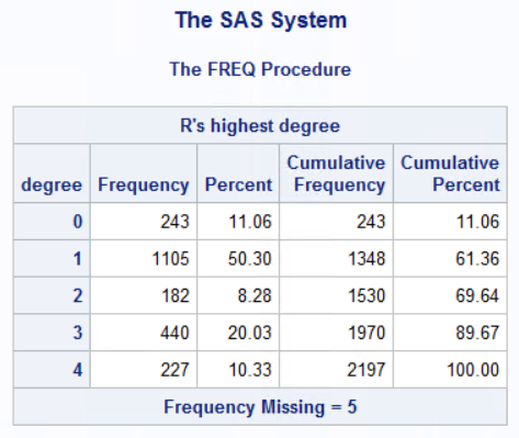
Exercise 3
Run a frequency for the the number of a respondent’s brothers and sisters, SIBS. (See Appendix A for answers.)
- What is the total number of cases?
- What is the number of missing cases?
- What percentage of respondents have only one sibling?
Proc Means
The proc means procedure generates a set of simple descriptive statistics for any numeric variable in a dataset. By default proc means will produce the mean, the number of non-missing values, the standard deviation, the minimum value, and the maximum value for each numeric variable.
A subset of variables can be specified with a var statement, otherwise SAS will produce statistics for all numeric variables in the dataset. For example, to request descriptive statistics for the variable realrinc, age, and hrs1:
proc means data = ourgss2018;
      var realrinc age hrs1;
run;
To specify the number of decimal places in the output, use the maxdec = n option where n is the number of decimal places. See an example of usage of the maxdec option below:
proc means data = ourgss2018 maxdec = 3;
      var realrinc age hrs1;
run;
Other statistics may be requested by adding keywords in the proc means statement after specifying the data set to be used. If other statistics are requested, the procedure will no longer produce the default statistics, they must also be requested.
For example, to request the mean, median, and range for the variable tvhours:
proc means data = ourgss2018 mean median range;
      var tvhours;
run;
The following is a table of the more common keywords used with proc means:
| Keyword | Statistic |
|---|---|
| clm | two-sided confidence limits |
| css | corrected sum of squares |
| cv | coefficient of variation |
| kurtosis | kurtosis |
| lclm | lower confidence limit |
| max | maximum value |
| mean | mean |
| min | minimum value |
| n | number of non-missing values |
| nmiss | number of missing values |
| range | the range |
| skewness | skewness |
| stddev | standard deviation |
| stderr | standard error of the mean |
| sum | the sum |
| sumwgt | sum of weight variables |
| uclm | upper confidence limit |
| uss | uncorrected sum of squares |
| var | variance |
| probt | probability of Student’s t |
| t | Student’s t |
| median (p50) | median |
| q1 (p25) | 25% quantile |
| q3 (p75) | 75% quantile |
| p1 | 1% quantile |
| p5 | 5% quantile |
| p10 | 10% quantile |
| p90 | 90% quantile |
| p95 | 95% quantile |
| p99 | 99% quantile |
Exercise 4
Use the proc means procedure to request the mean and standard deviation for the variables sibs and educ to 4 decimal places. (See Appendix A for answers.)
Proc Sort
Output for the proc means procedure can be computed for each level of another variable by adding a by statement to the procedure. The variable(s) named in the by statement are called “by variables”.
Before running proc means with a by statement, the data must first be sorted, using the proc sort procedure. For example, to report the occupational prestige score pres by academic degree levels group degree:
- Run a proc sort procedure to sort the data by degree.
proc sort data = ourgss2018;
      by degree;
run;
This will sort the data in ascending order by the variable degree.
- Next, run the proc means procedure, including the by statement.
proc means data = ourgss2018 mean;
      var pres;
      by degree;
run;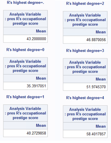
- The descriptive statistic, mean, is requested after specifying the dataset to be used.
- The var statement specifies that the descriptive statistic will only be calculated for the variable pres.
- The by statement specifies that a separate set of descriptive statistics will be calculated for each category of the variable degree, where (1) High School, (2) Junior College, (3) Bachelor, and (4) Graduate. The”.” represents missing
Exercise 5
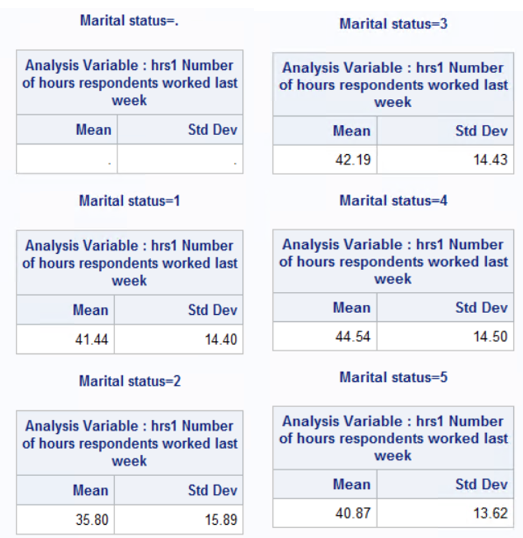
Use proc means to request the mean and standard deviation for the variable hrs1 broken down by marital status marital.
- Set the maximum number of decimal places to 2.
- Remember to use a proc sort statement to sort the data before running the proc means procedure.
(See Appendix A for answers.)
Proc Univariate
The proc univariate procedure generates statistics describing the distribution of variable(s). These statistics include the mean, median, mode, standard deviation, skewness, and kurtosis.
While these statistics must be requested when using proc means, all summary statistics are printed by default when using proc univariate.
Some additional options include:
- A subset of variables can be specified with a var statement, otherwise SAS will produce statistics for all numeric variables in the dataset. For example, to request summary statistics for the variable educ:
proc univariate data = ourgss2018;
      var educ;
run;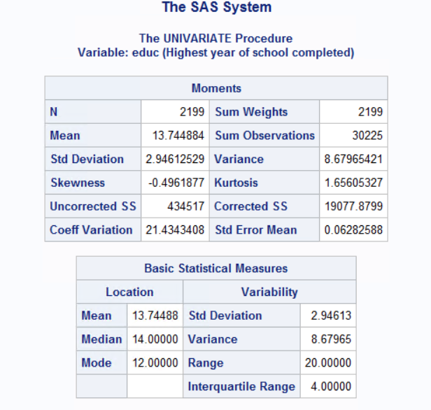
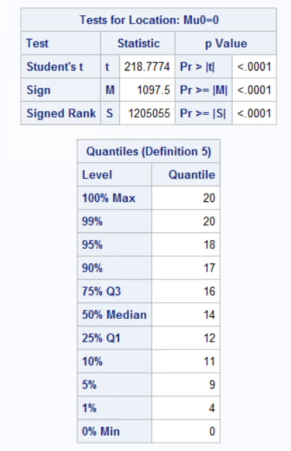
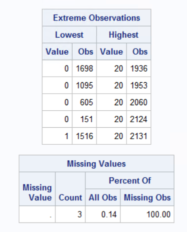
- The plot option produces three plots of the data (a stem-and-leaf plot, a box plot, and a normal probability plot).
- The normal option is used to request tests of normality.
- The by statement may be used to obtain separate analyses for by groups. Note: Remember to use proc sort first to sort the data in the order of the by variable(s).
Multivariate Tables
Contingency Tables
The proc freq procedure may also be used to produce contingency tables - crosstabulation and two-way tables - showing the joint distribution of two or more categorical variables, where the frequency distribution of one variable is subdivided according to the values of one or more variables, and the unique combination of values for two or more variables defines a cell.
A contingency table is produced using the proc freq procedure with the addition of an asterisk (*) between the two variables specified in a tables statement. For example, to generate a contingency table of the distribution of the variable postlife, where (1) indicates Yes - the respondent believes in life after death and (2) indicates No, and the variable sex, where (1) indicates the respondent is male and (2) indicates female:
proc freq data = ourgss2018;
      tables postlife*sex;
run;- The variable that appears immediately after the tables statement will appear in the rows.
- The variable that appears after the asterisk * will be placed in the columns.
- Either of the variables can go in the rows or columns.
Interpretation of a Contingency Table
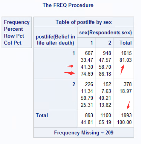
Number of valid cases: 1,993 cases are included in the table.
Number of missing cases: 209 cases do not have a valid value for at least one of the variables.
Note: Only valid values are included in the contingency table. A case with a missing value for at least one of the variables will be excluded from the table.
74.69 % of male respondents answered yes to the belief in life after death question.
Combining male and female, 81.03 % of respondents answered yes to the belief in life after death question.
Row 3 can be read as: 41.30 % of the respondents who answered yes to the belief in life after death question were male.
Some additional options that may be specified with proc freq. These are to be placed at the end of the table statement following a forward slash (/):
- list - Prints contingency tables in a list format rather than a grid
- missing- Includes missing values in frequency statistics
- nocol - Suppresses printing of column percentages
- norow - Suppresses printing of row percentages
- out = dataset_name - Writes the frequencies to a new dataset
- nofreq - Suppresses cell frequencies
- nopercent - Suppresses percentages
For example, the following syntax produces a contingency table in a list format:
proc freq data = ourgss2018;
      tables postlife*sex /list;
run;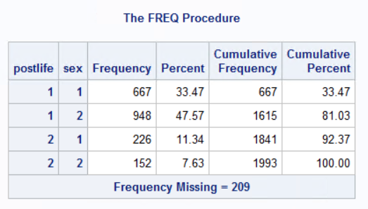
Exercise 6
To find out how many foreign-born and native-born survey respondents can speak a language other than English/Spanish, create a contingency table using the variables othlang, where (1) indicates Yes - the respondent can speak a language other than English/Spanish and (2) indicates No, and born, where (1) indicates Yes - the respondent was born in this country and (2) indicates No. (See Appendix A for answers.)
Graphics
Creating Charts
The proc gchart procedure may be used to create pie charts, vertical and horizontal bar charts, and histograms. One or multiple charts can be created in a single proc gchart procedure.
Bar Chart
A bar chart is a graphic representation of a categorical variable. It uses rectangles to show the frequency or proportion of each category of the variable in the data. A space is inserted in-between rectangles in order to differentiate a bar chart from a histogram (i.e., a graphic representation for a continuous variable).
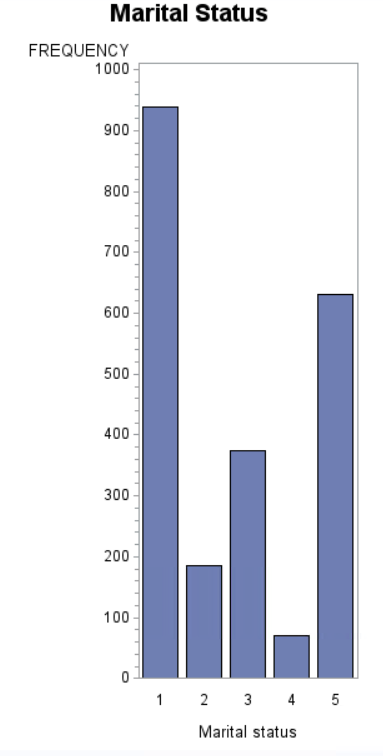
To create a vertical bar chart for the marital status of a respondent variable marital, use proc gchart with the variable of interest specified after a vbar statement.
proc gchart data = ourgss2018;
      title "Marital Status";
      vbar marital /discrete;
run;
quit;- The title statement is used to label the chart.
- The vbar statement produces a vertical bar chart for the variable marital.
- The discrete option is specified in the vbar statement to indicate that the variable contains discrete categories.
- The proc gchart procedure requires a quit statement to finish.
There are several additional options that may be used to change the appearance of the chart. The following options may be added to the vbar statement:
- cframe = x – Changes the background color, where x represents the color (e.g. red)
- ctext = x – Changes the color of the text, where x represents the color
- noframe – Removes the frame from the chart
- space = x – Specifies the distance between bars, where x represents the spacing
- width= x – Specifies the width of the bars, where x represents the width
The bar color may changed by using the additional statement: pattern color=bar x. This changes the color of the bars, where x represents the color.
To specify the statistic used to create the bar chart, add one of the following options to the vbar statement:
- freq – Uses the frequency in each discrete category
- percent – Uses the percent in each discrete category
A grouping variable may be used to produce separate bar charts, by using the additional statement group = grouping x. This uses the frequency in each discrete category of the variable represented by x.
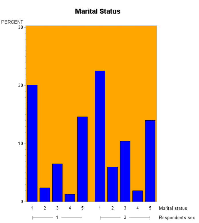
For example, to create a vertical bar chart of the percent in each category of marital with blue bars, an orange background, and grouped by sex:
proc gchart data = ourgss2018;
      title "Marital Status";
      vbar marital /discrete
             type = percent
             cframe = orange
             group=sex;
      pattern color=blue;
run;
quit;- The title statement is used to label the chart.
- The vbar statement produces a vertical bar chart for the variable marital.
- The discrete option is specified in the vbar statement to indicate taht the variable contains discrete categories.
- The percent option is specified to indicate that percent is that statistic that will be graphed.
- The cframe = orange option is specified to indicate that the background color will be orange.
- The group = sex option is specified to indicate that two sets of bars will be produced – one for men (sex=1) and the other for women (sex=2).
- The proc gchart procedure requires a quit statement to finish.
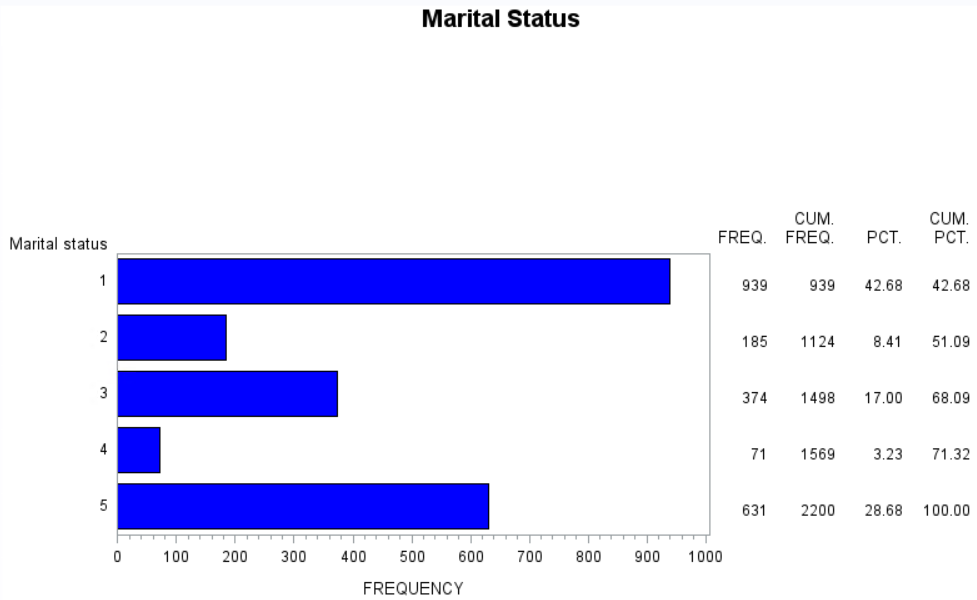
To create a horizontal bar chart use the hbar statement:
proc gchart data = ourgss2018;
      title "Marital Status";
      hbar marital /discrete ;
run;
quit;When a horizontal bar chart is created, the frequency distribution is printed to the right of the output.
Pie Chart
A pie chart is a graphic representation of a categorical variable, which uses a slice in a circle (or a pie) to show a frequency or a proportion of each category in the variable.
A pie chart is typically used to compare proportions. For example, a pie chart may be used to illustrate the proportional distribution of marital status.
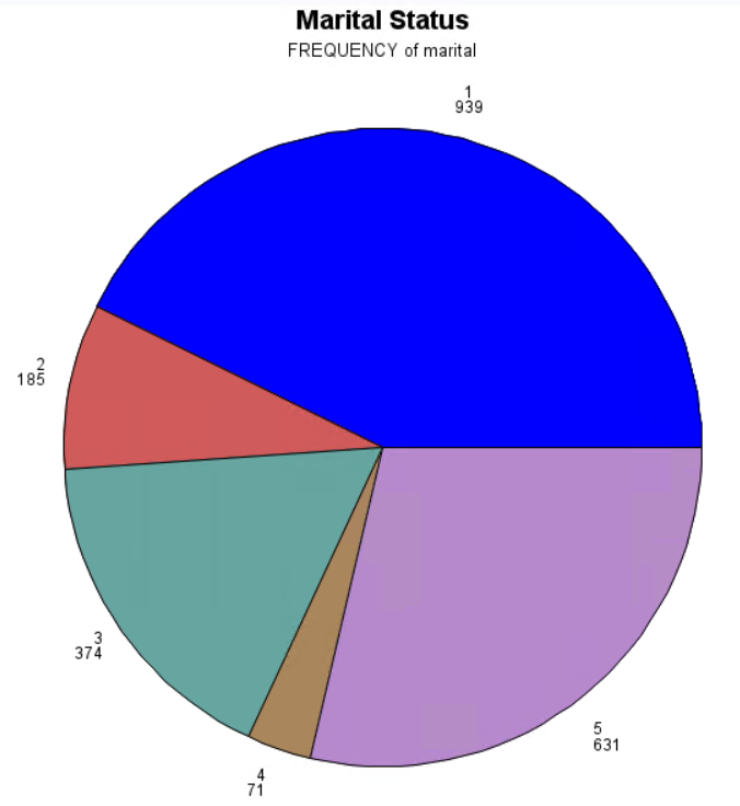
proc gchart data = ourgss2018;
      title "Marital Status";
      pie marital /discrete;
run;
quit;- The title statement is used to label the chart.
- The pie statement produces a pie chart for the variable marital.
- The discrete option is specified to indicate that the variable contains discrete categories.
- The proc gchart procedure requires a quit statement to finish.
There are several additional options that may be added to the pie statement to change the appearance of the chart:
ctext = text x – Changes the color of the text
slice = x – Indicates where the value label is placed in relation to the location of the pie slice, where x can be one of the following: arrow, inside, none, and outside.
The pie slice colors can be changed using an additional statement: pattern## c = x. This changes the color of the slice to the color, where x represents the number of the slice to be changed and the color to be used, respectively.
To specify the statistic used to create the pie slices, add one of the following options to the pie statement:
type = freq – Uses the frequency of each discrete category
type = percent – Uses the percent in each discrete category
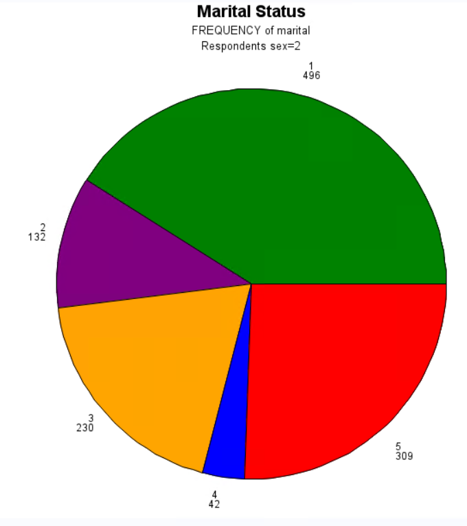
A grouping variable may be used to produce separate pie charts: group = grouping x. This creates a separate pie chart for each category of the grouping variable, represented by x.
For example, to create a pie chart of the percent in each category of the variable marital with green, purple, orange, blue, and red slices, grouped by sex:
proc gchart data = ourgss2018;
      title "Marital Status";
      pie marital /discrete
            group = sex;
      pattern1 c = green;
      pattern2 c = purple;
      pattern3 c = orange;
      pattern4 c = blue;
      pattern5 c = red;
run;
quit;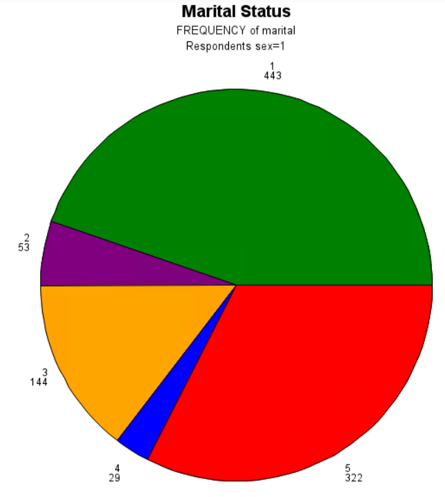
Exercise 7
Create a bar chart for the percent in each category of the variable neisafe. This variable is based on the question, How safe interviewer thinks neighborhood is? The answers are categorized as : Very Safe (1), Somewhat Safe (2), Somewhat Unsafe (3), or Very Unsafe (4). Use the title ``Belief in Neighborhood Safety’’. (See Appendix A for answers.)
Formatting Output
Adding Value Labels
Unlike other statistical programs, SAS does not label the numeric values of variables.
For example, in the frequency output for the variable marital, the numeric values 1-5 are shown, but there is no information about what each of these values stands for (i.e., 1 = Married and 2 = Widowed, etc.).
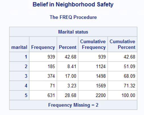
The value labels can be displayed in the output by using the proc format procedure. This procedure creates formats that will be associated with the variables specified later in a format statement. A series of value statements is used to indicate the value labels for each value of the variable.
To create value labels for the variable marital:
proc format;
    value maritalfmt
        1='Married'
        2 = 'Widowed'
        3 = 'Divorced'
        4 = 'Separated'
        5 = 'Never Married';
run;- The name of the format is specified as maritalFmt in the value statement.
- The values and labels are indicated in the series of value statements: value=’label’.
To apply the format when running a frequency procedure, include a format statement in the program:
proc freq data = ourgss2018;
    tables marital;
    format marital maritalfmt.;
run;- The format statement is organized so that the variable name marital appears immediately after format and is followed by the name of the format maritalFmt.
- When defining a new format with proc format, the format name cannot end in a period (.). However, when the format is applied to a variable in a format statement, the format name must end in a period.
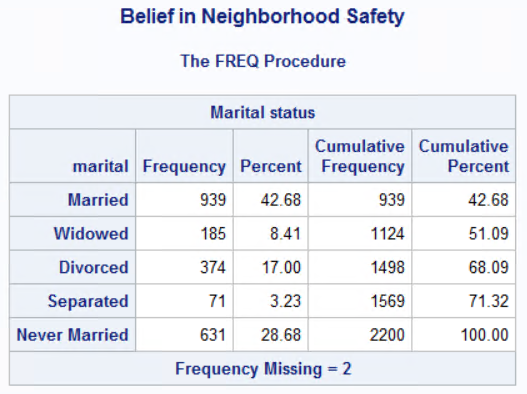
The frequency output is now labeled by the name of each category rather than the numeric value:
Saving and Printing
Your Data
We have discussed temporary and permanent datasets, and we’ve been working mostly with temporary libraries throughout this workbook.
The easiest way to save a dataset from the temporary work library is to use a datastep to create the same dataset in a permanent library:
data training.newgss2018;
    set ourgss2018;
run;
The Results Viewer
To save or print the entire contents of the Output window:
- Make the Results Viewer window active by clicking on it.
- Under the File menu, select either Save As or Print. SAS Output is saved with the extension .mht and can be opened in a web browser.
Images may also be exported from SAS on an individual basis:
- Fine the graph in the Results Viewer.
- Right-click on the graph and select Save picture as… from the menu.
The Program Editor
To save or print the contents of the Program Editor window:
- Make the Program Editor window active by clicking on it.
- Under the File menu, select either Save or Print. SAS programs are saved with the extension .sas
Opening SAS Programs
To open a pre-existing SAS Program double-click on the SAS Program in File Explorer or:
- Select File > Open Program.
- Navigate to the location of the program file on your computer.
- Highlight the program, and click Open.
The Log
To save or print the contents of the Log window:
- Make the Log window active by clicking on it.
- Under the File menu, select either Save or Print. SAS Logs are text files and are saved with the extension .txt.
Exiting SAS
Remember to save your data and output files before exiting the program.
Select File > Exit.
Appendix A: Answers to Exercises
Exercise 1
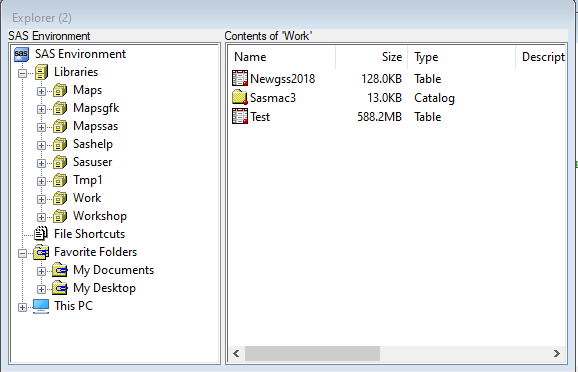
After submitting this program, observe what happens in the various windows of SAS:
- Editor: No changes.
- Log: The program statements will appear in the log, followed by notes about the number of observations that were read, how many observations and variables are included in the new dataset, and the amount of time it took to process the step.
- Explorer: A new dataset called NewGSS2018 will appear in the Work library.
Exercise 2
data ourgss2018;
      set newgss2018;
      if 0 <= degree <= 2 then bachelor_degree = 0;
      if 3 <= degree <= 4 then bachelor_degree = 1;
run;
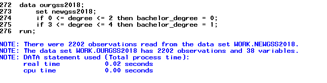
Verify in the Log window that the data step was performed and created a new dataset, ourgss2018, 2,202 observations and 38 variables.
Exercise 3
proc freq data = ourgss2018;
      tables sibs;
run;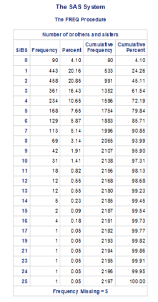
- The total number of cases is 2,197.
- The number of missing cases is 5.
- The percentage of respondents with only 1 sibling is 20.16
Exercise 4
proc means data = ourgss2018 mean stddev maxdec = 4;
      var sibs educ;
run;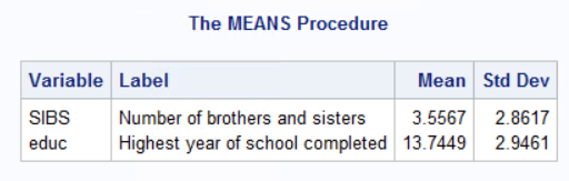
Exercise 5
proc sort data = ourgss2018;
      by marital;
run;

proc means data = ourgss2018 mean stddev maxdec = 2;
      var hrs1;
      by marital;
run;
The by statement here specifies that a separate set of descriptive statistics will be calculated for each category of the variable marital.
Exercise 6
proc freq data = ourgss2018;
      tables othlang*born;
run;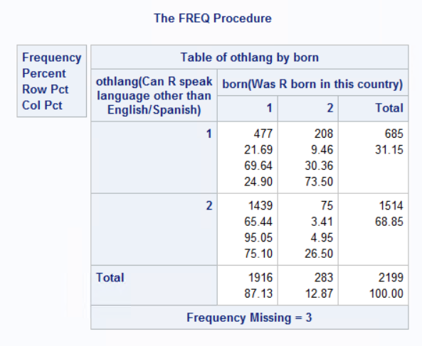
- 477 native-born respondents speak a language other than English/Spanish.
- 208 foreign-born respondents speak a language other than English/Spanish.
Exercise 7
proc gchart data = ourgss2018;
title "Belief in Neighborhood Safety";
vbar neisafe / discrete type=percent;
run;
quit;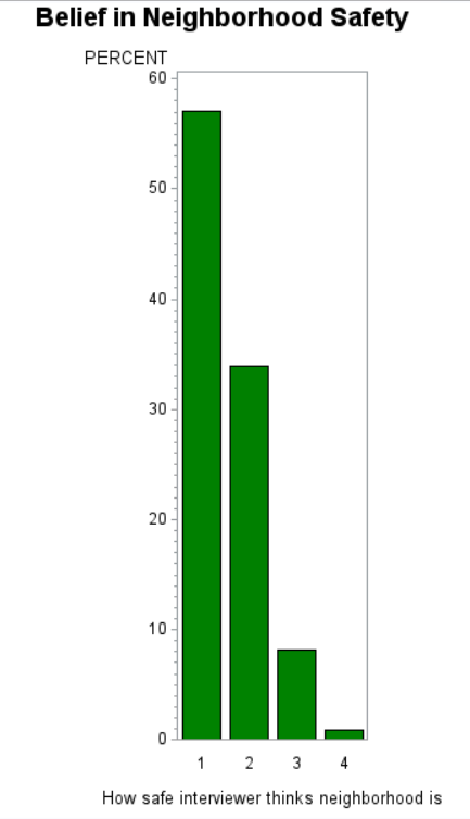
Appendix B: SAS Enhanced Editor Color Coding
- Data and proc statements are in bold navy.
- Other statements and options recognized by SAS are bright blue.
- Literal data that follows a datalines statement are highlighted yellow.
- Comments are green. - To comment, type an asterisk * at the beginning of the line and close the comment with a semicolon ;. - Comments can span multiple lines.
- Improper code is highlighted red.
- Variable and dataset names will remain black.
- Code in quotations is purple.
- Other numeric values SAS will read, such as the codes for column numbers and lengths/decimals of variable, are bold turquoise.