SPSS II

Inferential Statistics

After attending this training session, you will be able to run and interpret the following tests in SPSS:

1. Chi-square
2. Independent samples t-test
3. Levene’s test for the equality of variances
4. One-way ANOVA
5. Bivariate Statistics: Correlation
6. Bivariate Statistics: Regression
7. Multiple regression

Introduction

Code and Dataset

For this training session, please download the following data:

SPSS Workshop.sav

Recap of SPSS I

In the SPSS I training session, we covered the following topics. Please feel free to refer back to the SPSS I workbook using the following links if you would like a refresher.

• Starting SPSS
• The SPSS Environment
• Descriptive Statistics
• Data Transformation
• Multivariate Tables
• Graphics
• Saving and Printing

As in the SPSS I training session, we will be using data from the General Social Survey.

Loading the data

1. In the opening SPSS window click OK to Open an existing data source; an Open Data window will appear.
2. Navigate to and open the data file (SPSS Workshop.sav) you downloaded from our website. Please, communicate any problem you may have with the data during this training to the consultant or afterward to citl-statstraining@illinois.edu.

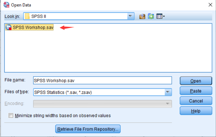
3. If you are unable to locate your data file, it is likely that the file is not in SPSS format. SPSS data files usually end in the suffix .sav so SPSS looks for these kinds of files first. If the data file is in a different format, change Files of type: to All files (.), and the file should appear. Double-click on the file and SPSS will open it if it is compatible with SPSS.

Note

Changing the extension of a file name to .sav does not convert the data file into an SPSS formatted data file. Rather, it must be imported through SPSS or another program for SPSS to be able to read it. Please contact CITL Data Analytics Group if you need assistance with this task.

Options

You may have noticed that after opening our data there are two windows popping up. The first window is the Data Editor interface, in which the data and variables are presented. The second window is the Output interface, in which all results of the computations will be presented. We are concentrating for now on the former as we have to specify some program settings. Let’s start changing the following options in the Data Editor window:

1. In the Menu bar, select Edit > Options.
2. In the General tab, under Variable Lists, select Display Names and Alphabetical.

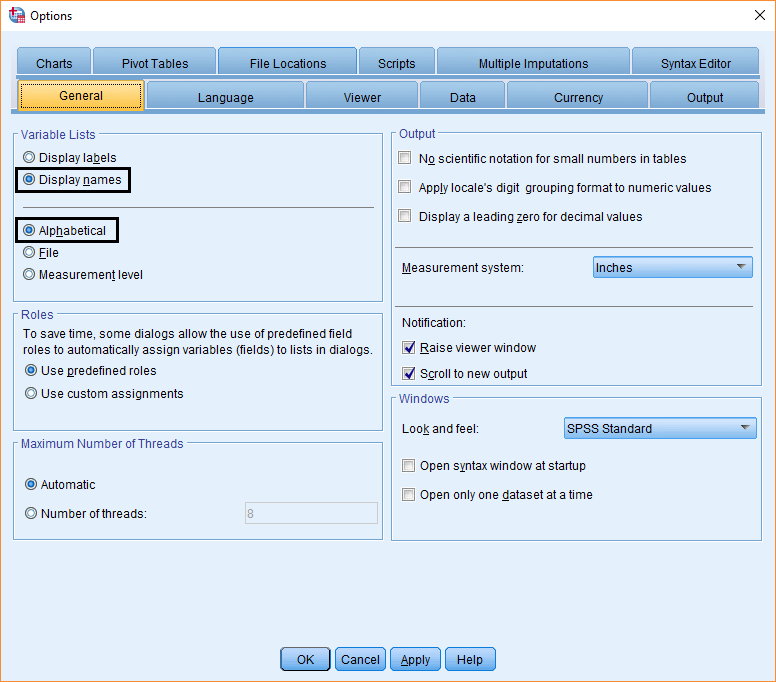
Note: These options change how the variables are displayed in the dialog boxes. They do not change the underlying data file in any way.

3. To change the labeling of the output so that both variable names and labels are displayed in output tables and graphs:

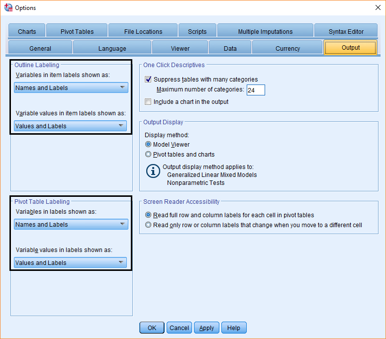
4. Click on the Output tab.
5. Under both Outline Labeling and Pivot Table Labeling, change the pull-down menus to specify Names and Labels or Values and Labels.

Now, click on the Pivot Tables tab and select the TableLook setting you prefer.

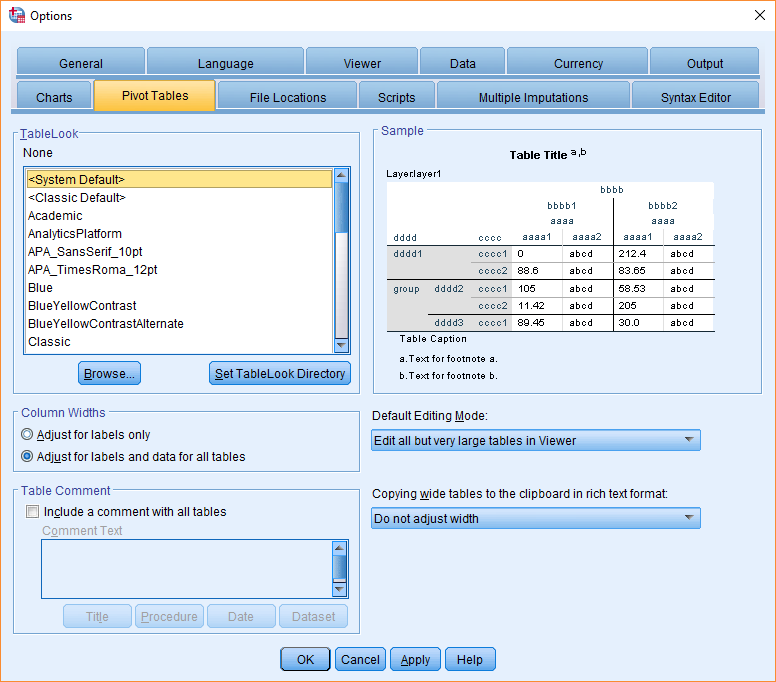
To display program commands in the output viewer: click on the Viewer tab, and select Display commands in log. This is useful when documenting your work.

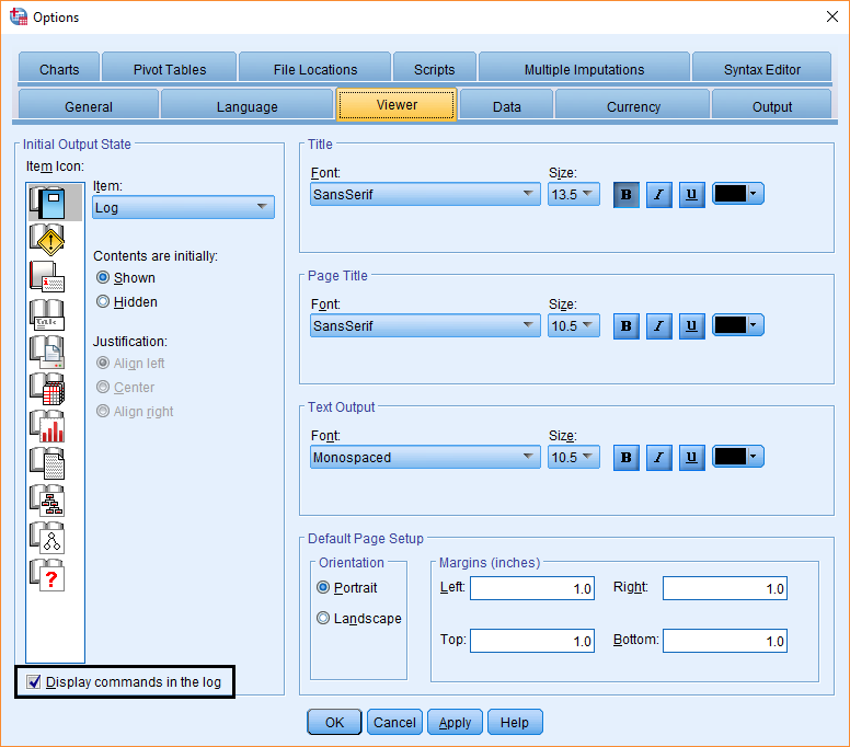
When you are done making changes, click Apply and then Ok to finish.

Chi-square test

A chi-square test is used to determine whether there is a statistically significant association between two categorical variables.

Example 1: 2x2 Table

For example, you may want to know if there is a significant association between the variables sex (Respondent’s gender) and hschem (Respondent ever took chemistry class in high school). The chi-square test statistic is requested in the Crosstabs procedure.

1. In the Menu bar, select Analyze > Descriptive Statistics > Crosstabs.
2. Move the dependent variable hschem into Row(s) and the independent variable sex into Column(s).
3. Click Cells, select Column for Percentages and select Expected for Counts, and click Continue.

When selecting whether you want column or row percentages, select whichever contains the independent variable. In this case, our independent variable sex is in the column, so select column percentages.

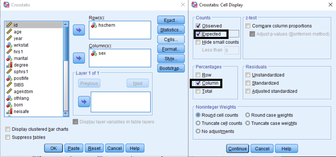
4. Click Statistics, and select Chi-square.

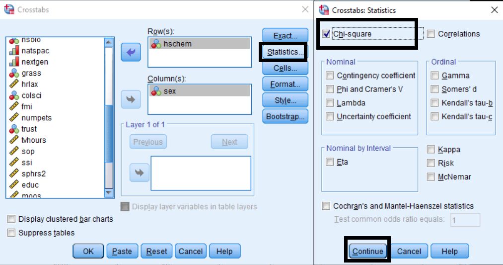
5. Click Continue and OK to finish.

Interpretation of Output: The following three tables are created after requesting a crosstabulation table with the chi-square test statistic.

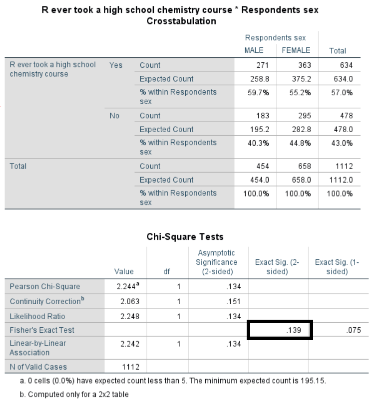
SPSS generates the following test statistics for chi-square:

Note

The levels of measurement, the number of categories within the variables, and the sample size will determine which test statistic is appropriate.

• Pearson Chi-Square: Used to test the hypothesis that the row and column variables are independent. This should not be used if any cell has an expected value less than 1, or if more than 20$
  
• Continuity Correction: This correction is applied in the computation of chi-square for 2x2 tables to improve the approximation. Corrected chi-square values are always smaller than uncorrected values.
• Likelihood Ratio: A goodness-of-fit statistic similar to Pearson’s chi-square, this statistic is appropriate to report for smaller sample sizes. The likelihood ratio approaches the Pearson’s chi-square as n increases, so for large sample sizes, the two statistics are the same and either can be reported.
• Fisher’s Exact Test: A test for independence in a 2x2 table. This statistic is most useful when the total sample size and expected values are small.
• Linear-by-Linear Association: A measure of the linear association between the row and column variables. It is also referred to as the Mantel-Haenszel chi-square and the Mantel-Haenszel test for linear association. Note: This statistic should not be used for nominal data.

Because this example uses a 2X2 table, we will use Fisher’s Exact test. Here, the Fisher’s Exact test has a probability of 1.139 that the null hypothesis is true, so we fail to reject the null hypothesis (using two-tail, as gender’s value doesn’t represent the actual quantity). Thus, we can conclude that there is NO statistically significant relationship between the respondents’ sex and taking a chemistry class in high school.

Example 2: More than 2X2 Table

In this example, we want to know if there is a significant association between the dependent variable natspac (attitude towards the space exploration program) and the independent variable colsci (whether respondents took college-level science courses). It should produce a crosstab analysis for a 2X3 Table.

1. In the Menu bar, select Analyze > Descriptive Statistics > Crosstabs.
2. Move the dependent variable nextspac into Row(s) and the independent variable colsci into Column(s).
3. Click Cells, select Column for Percentages and and select Expected for Counts, and click Continue.
4. Click Statistics, and select Chi-square.

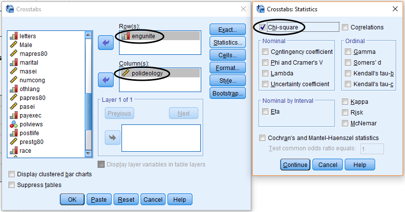
5. Click Continue and OK to finish.

Interpretation of Output:

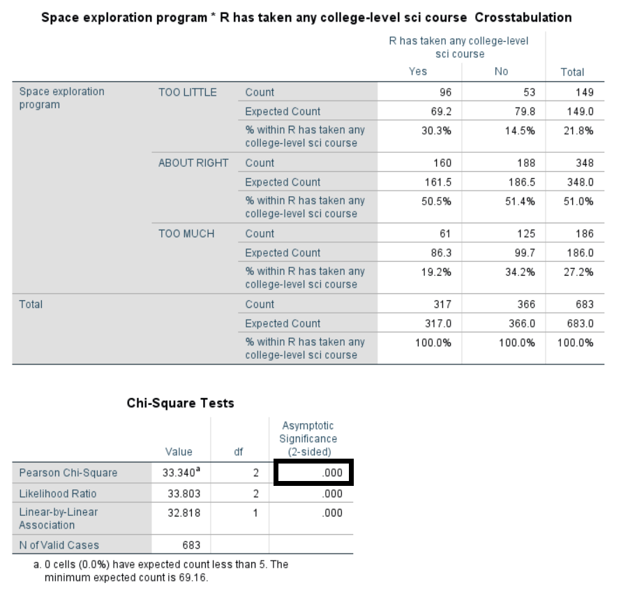
Because 0 cells have expected counts less than 5, it is appropriate to use the Pearson Chi-Square test statistic in this example. The level of significance is 0.000. Therefore, it may be concluded that there is a statistically significant relationship between attitudes towards the space exploration program and those who took college level science classes.

Tip

Measures of the strength of the association can be requested in addition to the Chi-Square statistic in the Crosstabs: Statistics dialog box.

Exercise 1

Perform a chi-square test to determine if the variable degree (Respondent’s highest degree) is significantly associated with the variable grass (belief that marijuana should be legal). 1. How many high school graduates said “Yes” to legalization? 2. Is there a statistically significant relationship between the two variables? Which chi-square test statistic is appropriate?

(See Appendix A for answers.)

Independent Samples T Test

An independent samples t-test determines whether there is a statistically significant difference in the mean of a continuous dependent variable between two groups.

For example, this procedure may be used to find out if there is a statistically significant difference between the responses of men and women (sex) for how much they have to relax per day (hrlax). 1. In the Menu bar, select Analyze > Compare Means > Independent Sample T Test. 2. Place the dependent variable hrlax into the Test Variable(s) box. 3. Place the variable sex in the Grouping Variable box.

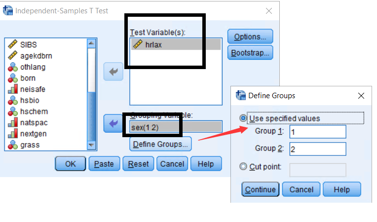
4. Click on Define Groups and set Group 1 = 1 (Male) and Group 2 = 2 (Female).
5. Click Continue and OK.

Note

To determine how the grouping variable is coded, generate a frequency table of the variable or in the Independent-Samples T Test dialog box, right-click the grouping variable, and select Variable Information.

The two independent samples t-test generates two output tables.

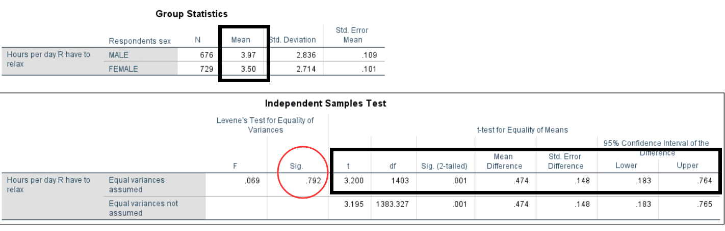
The Group Statistics table provides descriptive statistics of the independent variable for each group. According to the statistics in this box, males have to relax 3.97 hours per day while women have to relax 3.50 hours per day.

The Independent Samples Test table is used to decide whether there is a statistically significant difference by sex in beliefs about how much corporate heads make.

There are two sets of statistics generated by SPSS:

• Equal variances assumed: Assumes that the variances in the distribution of the dependent variable are equal for both groups.
• Equal variances not assumed: Does not assume that the variances in the distributions are equal.

To determine which statistics are appropriate, check the significance level for Levene’s Test for Equality of Variances, located in the output table for the independent samples t-test. This tests the null hypothesis that the variances are equal.

Because the significance of Levene’s test in this example is larger than 0.05, we fail to reject the null hypothesis, and the assumption of equal variance is met. In such a case, the statistics for Equal variances assumed should be used.

The significance level of the t-statistic is less than 0.05, therefore you may conclude that there is a statistically significant difference in the number of hours men and women have to relax per day.

Exercise 2

Find out if there is a statistically significant difference in terms of family income (fmi)between respondents who took college-level science courses and those who didn’t (colsci). (See Appendix A for answers.)

ANOVA

A One-way ANOVA is used to determine whether there is a statistically significant difference in the mean of a continuous dependent variable among more than two groups.

For example, this procedure may be used to find out if there is a statistically significant difference in the number of hours spent watching TV (tvhours) based on marital status (marital).

1. In the Menu bar, select Analyze > Compare Means > One-Way ANOVA.
2. Place the dependent variable tvhours into the Dependent List and the independent variable marital into the Factor box.

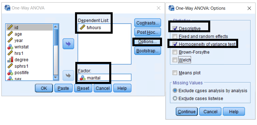
3. Click on Options, and select Descriptive and Homogeneity of Variance Test.
4. Click Continue and OK to finish.

First Step of Interpreting ANOVA Output: Levene Test

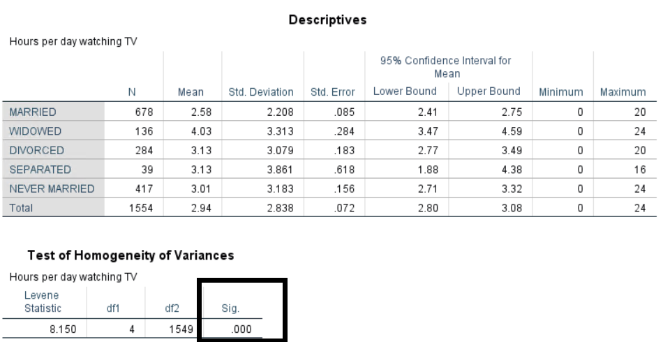
As the significant threshold is 0.05 generally, the Levene’s Test of Homogeneity of Variances is smaller than this threshold and thus significant (\(p = 0.000\)). As seen in the second output table, we reject the null hypothesis that the variances are equal, and not-equal variances are assumed. This is important in determining which F-test will be used and which post hoc tests will be best suited for any further analysis.

Second Step of Interpreting ANOVA Output: Choose Test

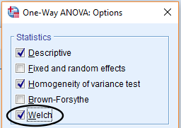
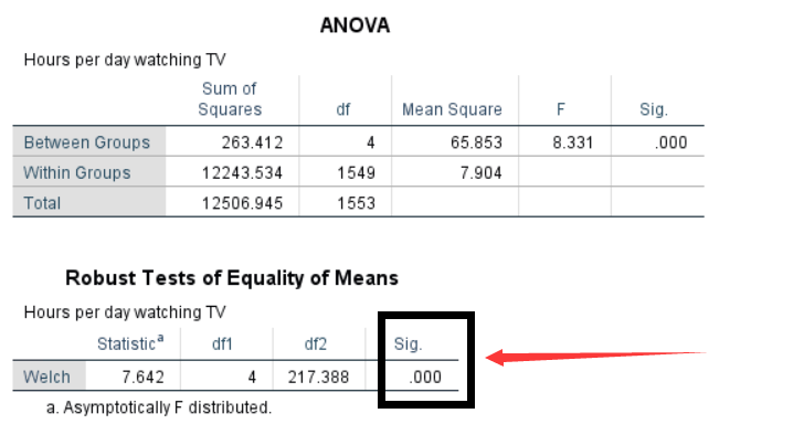
When Levene’s test shows that the variances are not homogeneous, choose the Welch test of equality of means to report ANOVA results. To request this test, select Options in the One-Way ANOVA dialog box, select Welch, and click Continue. This will generate the Robust Tests of Equality of Means table, which gives a more accurate significance level than the default F-test. In this case, \(p = 0.000\) for Welch Test, therefore we conclude that there are significant differences in the number of hours spent watching TV based on marital status. If the variances are found to be homogeneous following the Levene’s test, we should otherwise choose the regular ANOVA table with homogeneous options.

ANOVA Post Hoc Tests

While the ANOVA procedure itself determines whether differences exist among the group means, post hoc tests are needed to determine which means differ, and which post hoc test you use depends on the homogeneity of the variances.

As we found above, when looking at differences in number of TV hours watching per day (tvhours) by marital status in people (marital), equal variances cannot be assumed. Therefore, we must select a post hoc test that assumes not-equal variances.

1. In the Menu bar, select Analyze > Compare Means > One-Way ANOVA.
2. In the One-Way ANOVA dialog box, click Post Hoc, and select Games-Howell.

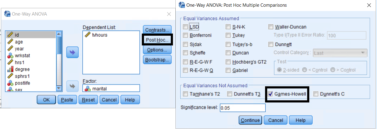
3. Games-Howell is a pairwise test – Pairwise tests compare the differences between each pair of means – with the null hypothesis that the paired means are equal.

4. Click Continue and OK to finish.

Note

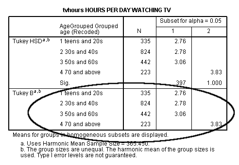
If equal variances can be assumed, you should select the Tukey or Tukey’s-b post hoc test.

Multiple Comparisons

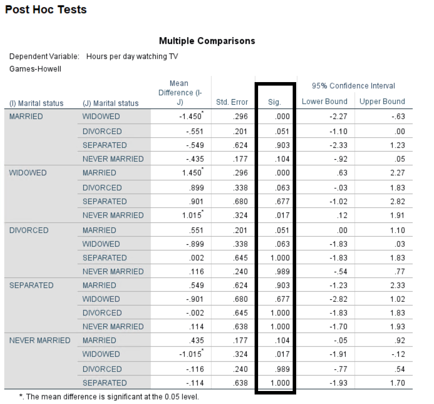
The Multiple Comparisons table provides the results of the Games-Howell post hoc test.

From this table it may be concluded that:

1. Group Married mean is significantly different from the group Widowed mean.
2. Group Widowed mean is significantly different from group Never Married mean.
3. All the other groups based on marital status have no significant difference from each other.

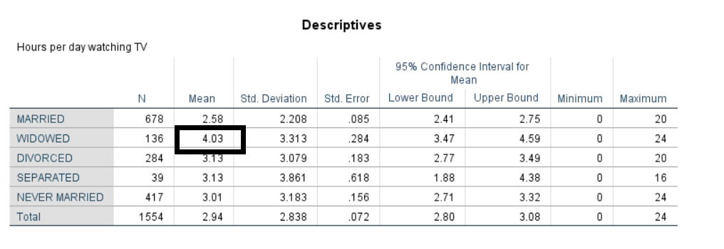
After identifying statistically significant differences, look back at the table of descriptive statistics to determine which marital groups spend more (or less) time watching TV per day. It is clear that the mean hours of time spent watching TV per day is significantly higher for group Widowed.

Homogeneous Subsets

Exercise 3

Using the One-Way ANOVA procedure, find out whether the mean level of family income (fmi) is different among different education groups (degree). Remember to check the homogeneity of variances. (See Appendix A for answers.)

Bivariate Correlation

Correlation is a measure of the linear relationship between two continuous variables. A correlation coefficient ranges from -1 to 1. A positive correlation coefficient indicates that there is a positive linear relationship. On the other hand, a negative correlation coefficient indicates that there is a negative linear relationship. A correlation coefficient of 0 indicates that there is no linear relationship between two variables.

For example, this procedure may be used to measure the relationship between the continuous variables spouse occupation prestige score (sop), spouse socioeconomic index score (ssi), and number of hours the spouse usually works a week (sphrs2).

Note

A bivariate correlation is used to determine the relationship between only two continuous variables.

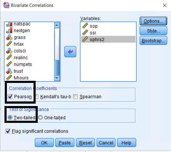
1. In the Menu bar, select Analyze > Correlate > Bivariate.
2. In the Bivariate Correlations dialog box, move the variables sop, ssi, and sphrs2 to the Variables: box.

3. Click OK to finish.

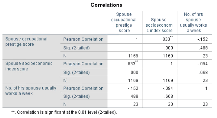
Each cell contains:

• a correlation coefficient (Pearson Correlation),
• the p-value associated with the correlation coefficient (Sig.),
• the number of cases (N).

The footnote below the correlation table defines the level of significance associated with an asterisk - the more asterisks displayed, the higher the level of significance.

In this example, the correlation coefficient between sop and ssi is 0.833 and the significance of the coefficient is 0.000, which suggests that these two variables are significantly and positively correlated.

Note on the number of cases (N): According to the third row of the cell for the correlation of sop and ssi, 1,169 valid cases are used. The correlation of sphrs2 and ssi or sop only used 23 valid cases.

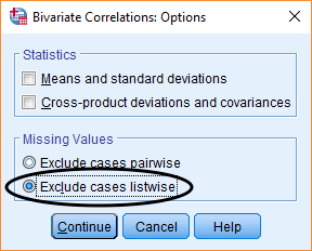
The default treatment of missing cases in the Correlation procedure is to use the maximum number of non-missing values for each pair of variables. This is known as pairwise deletion.

An alternative treatment of missing cases is listwise deletion, which can be enabled by clicking Options in the Bivariate Correlations dialog box. When this option is selected, cases with a missing value in any of the variables will be excluded from the analysis. Thus, when only two variables are included, the sample size is the same whether pairwise or listwise deletion is used. However, these options make a difference in the sample size when three or more variables are included. Note that the interpretation of the correlation coefficient for listwise deletion is the same as that for pairwise deletion.

Exercise 4

Measure the association between the variables highest year of school completed (educ), respondent’s father’s occupational prestige index (faos) and respondent’s mother’s occupational prestige index (moos), once using pairwise deletion and again using listwise deletion, to compare how the sample size changes. (See Appendix A for answers.)

Bivariate Regression

Bivariate regression is used to assess the effect of a continuous or dichotomous independent variable on a continuous dependent variable. This example uses bivariate regression to measure the effect of respondent’s age (age) on respondent’s income (realrinc).

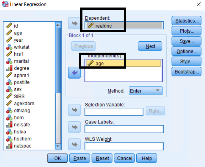
1. In the Menu bar, select Analyze > Regression > Linear.
2. Place realrinc into the Dependent box and age into the Independent(s) box.

3. Click OK to finish.

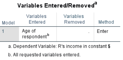
The regression procedure generates four tables: Variables Entered/Removed, Model Summary, ANOVA, and Coefficients.

• The Variables Entered/Removed table lists the independent variable included in the model. Only one independent variable, age, was included in this model.

• The Model Summary table provides information about the overall fit of the model.

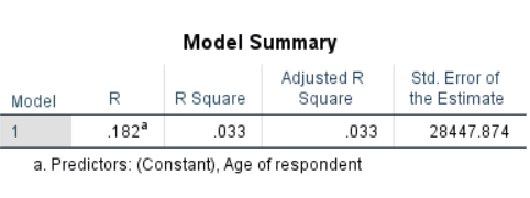
• R (aka Pearson’s R) is the correlation between the dependent variable and independent variable. In this example, income and age are positively correlated.
• R square (aka the coefficient of determination) tells you the proportion of variation in the dependent variable explained by the independent variable. R square ranges from 0 (no effect of an independent variable on a dependent variable) to 1 (perfect prediction of dependent variable by given independent variable).
  • In this example, 3.3% of the variation in income (dependent variable) is explained by the age (independent variable).
• Adjusted R square is adjusted for the number of independent variables used in the model. However, since there is only one independent variable in this example, the R square and Adjusted R square are the same.

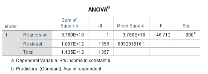
The ANOVA table measures whether the independent variable reliably predicts the dependent variable. In this example, the F statistic is statistically significant (\(p< 0.05\)). Thus, age is a significant predictor of income.

• The Coefficients table provides the values of the unstandardized regression coefficients (B), standardized coefficients (Beta), and a significance test of the coefficients (Sig.).

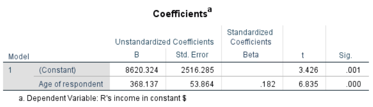
The regression coefficient for the constant is 8620.324 and the unstandardized coefficients for the independent variable educ is 368.137. From this, it can be said that the predicted level of income will increase by $368.137 for each additional year of age. Because this effect is measured in the original scale of the dependent variable, it is referred to as an unstandardized coefficient. Thus, when you have multiple independent variables measured in the different units in the model, you cannot compare the effects of independent variables using unstandardized coefficients. This will be addressed further in the section on Multiple Regression.

The standard error (Std. Error) is used to calculate the t-value (t). This statistic is used to test the null hypothesis that the unstandardized coefficient is equal to 0. In this example, age is statistically significant at the 0.000 level. This means that you can reject the null hypothesis that the age variable’s coefficient is equal to 0 and conclude that age is a significant predictor of income.

Exercise 5

Does independent variable age (age) affect dependent variable of performance on a vocabulary test (wordsum)? (See Appendix A for answers.)

Multiple Regression

Multiple regression is used to assess the effect of more than one continuous or dichotomous independent variable on another continuous dependent variable. Multiple regression is the same as bivariate regression, except it uses two or more independent variables to explain the variation of the dependent variable. This example uses multiple regression to measure the effect of respondent’s occupational prestige score (pres) and age (age) on respondent’s income (realrinc).

1. In the Menu bar, select Analyze > Regression > Linear.
2. Place realrinc into the Dependent box and pres and age into the Independent(s) box.

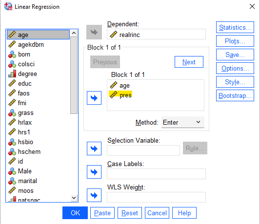
3. Click OK to finish.

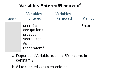
The regression procedure generates four tables: Variables Entered/Removed, Model Summary, ANOVA, and Coefficients.

• The Variables Entered/Removed table lists the independent variables included in the model. Two independent variables, pres and age, were included in this model.

• The Model Summary table provides information about the overall fit of the model. Since the denominator of R-square is fixed, each additional variable used in the equation can only increase the size of the numerator. As a result, the introduction of additional variables produces a higher R square value, regardless of the efficiency of the model.

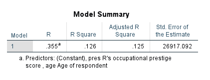
Since R Square will never decrease by adding more independent variables into the model, some researchers report an Adjusted R Square, which corrects this bias by adjusting both the numerator and the denominator by their respective degrees of freedom. Adjusted R Square is calculated using the equation below, where n is the number of observations and k is the number of independent variables.

\[ \text{Adjusted } R^2 = 1 - (1 - R)^2 \times \frac{n - 1}{n - k - 1} \]

Unlike R Square, the Adjusted R Square can decline in value. It is important to keep in mind, however, that the R Square value is a proportion, while the Adjusted R Square is not. Therefore, after adding one independent variable, the Adjusted R Square may decrease while the R Square may increase. If the Adjusted R Square is much lower than the R Square, this usually indicates that some relevant explanatory variables are not specified in the model.

In this example, compared to the bivariate model in the previous section, both R Square and Adjusted R Square have increased. Hence, this new model explains more variation of the dependent variable than the old model with one independent variable.

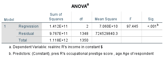
• The ANOVA table measures whether the independent variables significantly predicts the dependent variable. In this example, the F statistic is below 0.05. Thus, respondent’s occupational prestige score and age are significant predictors of income.

• The Coefficients table provides the values of the unstandardized regression coefficients (B), standardized coefficients (Beta), t-test statistics (t), and p-values (Sig.). It shows that a unit increase in age will increase predicted income by $285.290 while holding the occupational prestige score constant. The t-test statistic is 5.534, and the p-value associated with the t-test statistic is .001. Thus, age is statistically significant while controlling for pres. Likewise, a unit increase in pres will decrease the predicted income by $635.071 while holding age constant. The t-test statistic is 11.981, and the p-value associated with the t-test statistic is .001. Hence, pres is statistically significant while controlling for age.

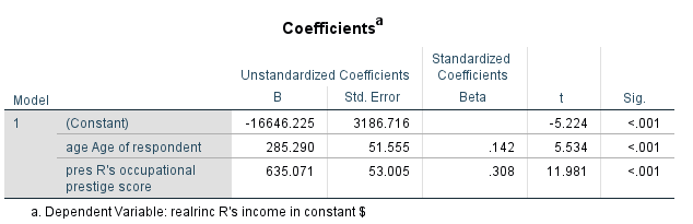
To compare the magnitude of the effect of each independent variable, the coefficients must be standardized using the same scale. The standardized coefficient (Beta) measures change in the dependent variable (measured in standard deviations) per one standard deviation change in the independent variable. Predicted income will increase by 0.142 standard deviation units for each one standard deviation increase in age while it will increase 0.308 standard deviation units for each one standard deviation increase in pres. Because the standardized coefficient for pres is larger than that for age we can conclude that occupational prestige has a larger impact on real income than age.

Exercise 6

Does the occupational prestige of a respondent’s parents (faos and moos) and respondent’s sex (Male) affect the respondent’s occupational prestige (pres)? (See Appendix A for answers.)

Appendix A: Answers for Exercises

Exercise 1

1. In the Menu bar, select Analyze > Descriptive Statistics > Crosstabs.
2. Move the dependent variable grass into Row(s) and the independent variable degree into Column(s).

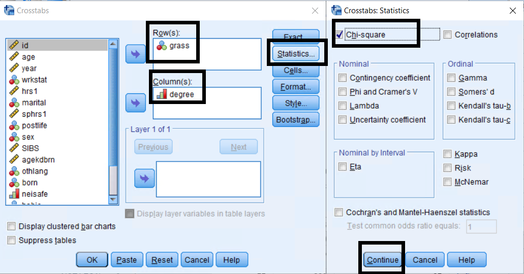
3. Click Cells, select Column for Percentages, and click Continue.
4. Click Statistics, and select Chi-square.
5. Click Continue and OK to finish.

Results:

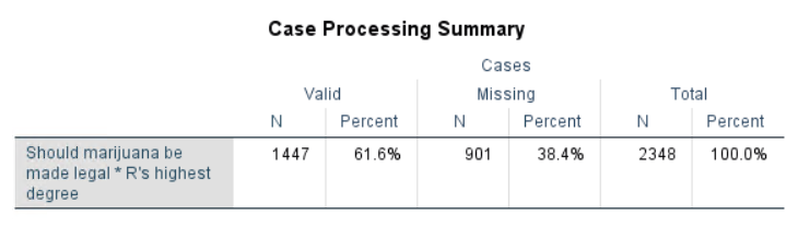
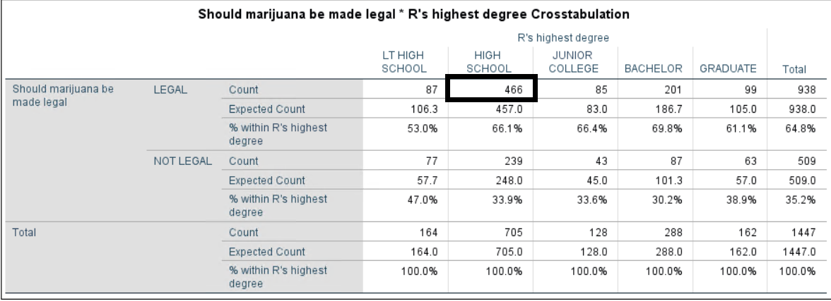
1. 466 high school graduates said Yes to legalization.
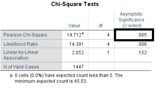
2. All expected cells are larger than 5, so we should use Pearson Chi-Square. The p-value associated with the Pearson chi-square statistic (0.005) is less than 0.05. Thus, there is a statistically significant relationship between the two variables.

Exercise 2

1. In the Menu bar, select Analyze > Compare Means > Independent Sample T Test.
2. Place the dependent variable fmi into the Test variable(s) box and the variable colsci in the Grouping variable box.

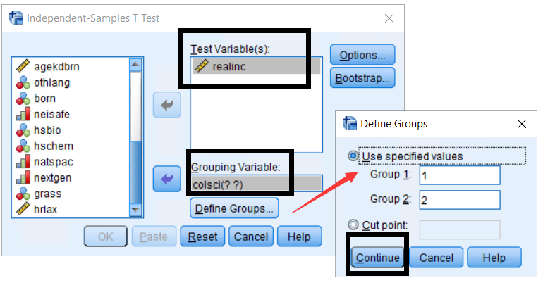
3. Click Define groups and set Group 1 = 1 (Yes) and Group 2 = 2 (No).
4. Click on Continue, and OK.

Results:

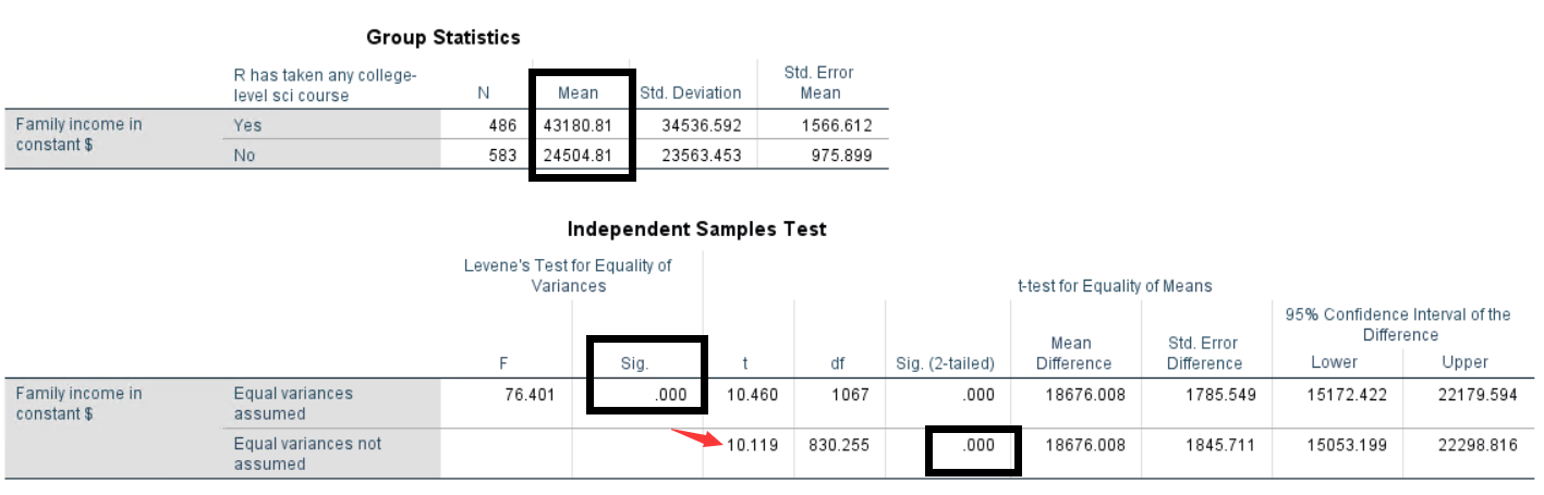
• Because the Levene’s Test for Equality of Variances is significant (\(p < 0.05\)), the Equal variances not assumed test statistic is appropriate to use.
• The t-test statistic (10.119) is significant (\(p < 0.05\)), therefore the amount of family income significantly differs based on if they took or didn’t take college-level science courses.

Exercise 3

1. In the Menu bar, select Analyze > Compare Means > One-Way ANOVA.
2. Place the dependent variable fmi into the Dependent List and the independent variable degree into the Factor box.

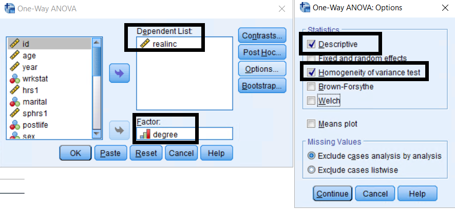
3. Click Options and select Descriptive and Homogeneity of Variance Test.
4. Click Continue and OK to finish.

Results:

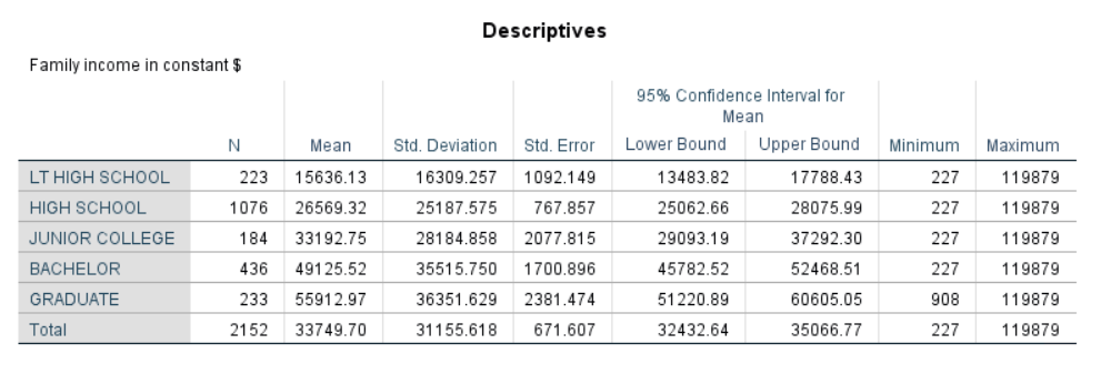
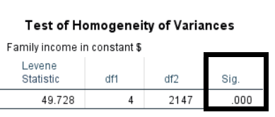
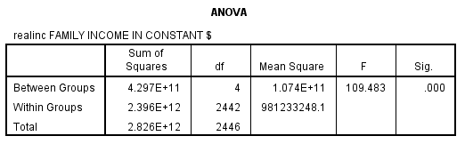
Because the Test of Homogeneity of Variances is significant the homogeneity of variances assumption is not met, and the ANOVA procedure will have to be run a second time, requesting the Welch test under Options in the One-way ANOVA dialog box. This will generate the Robust Tests of Equality of Means table.

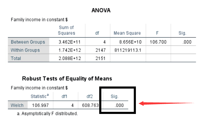
From the output, you can conclude that differences in average income among educational groups are statistically significant.

To conduct a Post Hoc Test to determine which means differ:

1. In the Menu bar, select Analyze > Compare Means > One-Way ANOVA.
2. Place the dependent variable fmi into the Dependent List and the independent variable degree into the Factor box.
3. In the One-Way ANOVA dialog box, click Post Hoc.
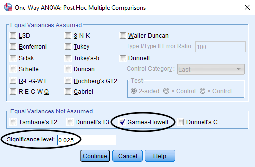
4. Change the Significance level from 0.05 to 0.25 for the sake of this example.
5. Because the results of the Test of Homogeneity of Variances is significant (\(p < 0.05\)), you must select the Games-Howell post hoc test. This test does not assume equality of variances.

6. Click Continue and OK to finish.

Results:

The Multiple Comparisons table provides the results of the Games-Howell post hoc test. From this table it may be concluded that:

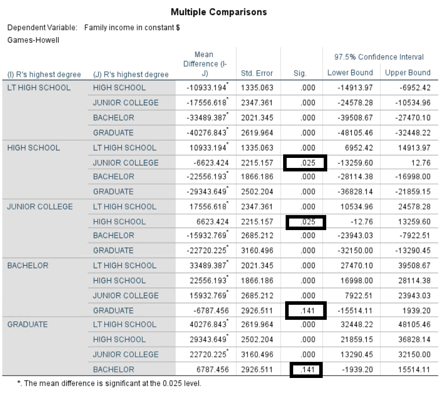
1. Group Less than High School is significantly different from all other groups at the 0.025 level.
2. Group High School is significantly different from all other groups except group Junior College at the 0.025 level.

More specifically, those with a high school degree make $10,933.194 more in family income than those with less than a high school education, but the -$6,623.424 difference in family income between those with a high school degree and those with a junior college education is not significant. 3. Group Junior college is significantly different from all other groups except group High school at the 0.025 level. 4. Group Bachelor is significantly different from all other groups except group Graduate (and vice versa) at the 0.025 level.

Exercise 4

Correlation with Pairwise Deletion:

1. In the Menu bar, select Analyze > Correlate > Bivariate.
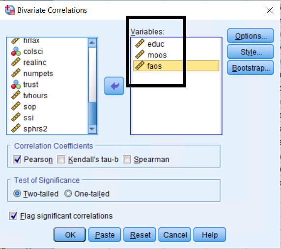
2. In the Bivariate Correlations dialog box, move the variables educ, faos, and moos to the Variables box.

3. Click Continue and OK to finish.
   

Correlation with Listwise Deletion:

1. In the Menu bar, select Analyze > Correlate > Bivariate.
2. In the Bivariate Correlations dialog box, move the variables educ, faos, and moos to the Variables box.

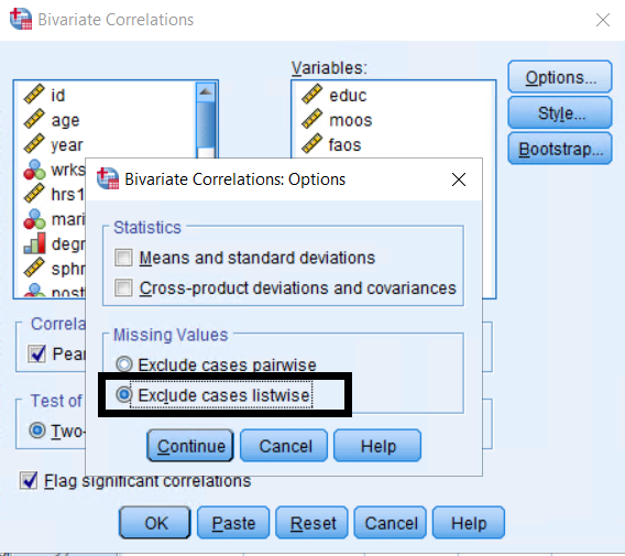
3. Click Options, and select Exclude cases listwise.
4. Click Continue and OK to finish.

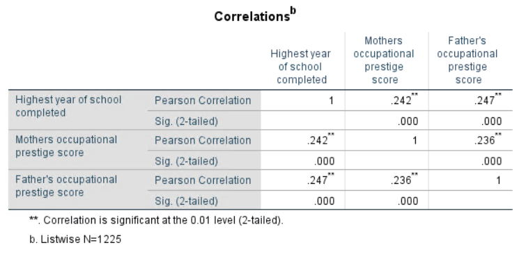
Results:

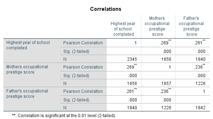
• Educational attainment (educ) is significantly and positively correlated with mother’s and father’s occupational prestige score (moos and faos) at the 0.01 level.
• Mother’s and father’s occupational prestige score are also significantly and positively correlated with each other at the 0.01 level.
• While the direction and strength of the relationship do not change significantly if you use either pairwise or listwise deletion, the absolute value of the correlation coefficient does change depending on the treatment of missing cases.

Exercise 5

1. In the Menu bar, select Analyze > Regression > Linear.
2. Place wordsum into the Dependent box and age into the Independent(s) box.

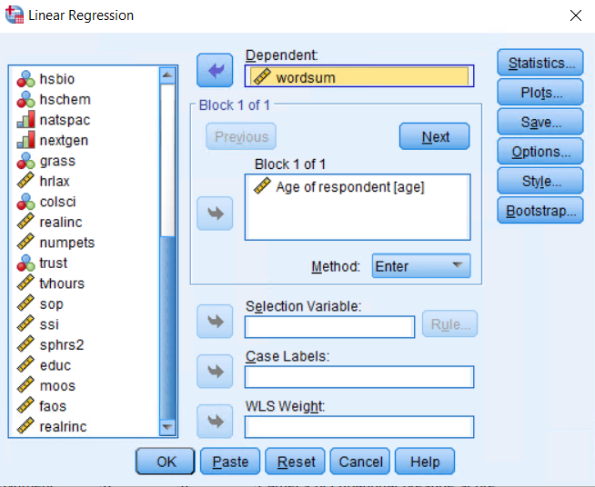
3. Click OK to finish.

Results:

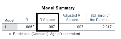
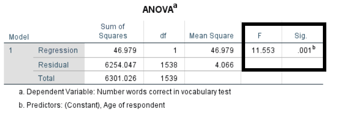
• The R Square is 0.007, meaning age can explain 0.7% of variation in the number of words correct in vocabulary test.
• Because the F statistic is statistically significant, age is a significant predictor of vocabulary test score.
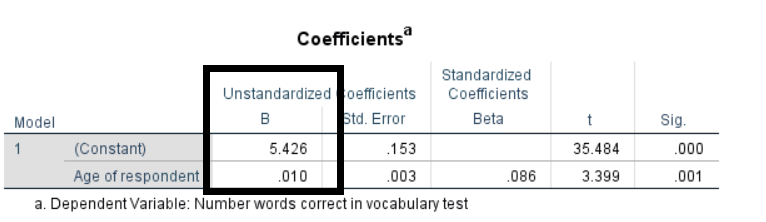
• The regression coefficient for the constant is 5.426, and the one for the independent variable age is 0.010. The predicted vocabulary test score will increase by 0.010 for each additional year of age.
• The effect of age on wordsum is statistically significant at the 0.01 level.

Exercise 6

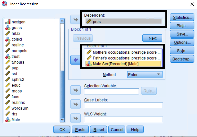
1. In the Menu bar, select Analyze > Regression > Linear.
2. Place pres into the Dependent box and faos, moos, and Male into the Independent(s) box.

3. Click OK to finish.

Results:

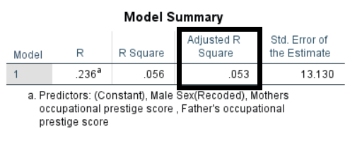
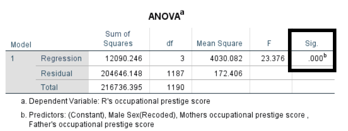
• Regression result yields an adjusted R-squared of 0.53 and an R-squared of 0.56.It means that 56% of variance in respondent’s occupational prestige score can be explained by mother’s occupational prestige score, father’s occupational prestige score, and sex.
• Because the F statistic is statistically significant, mother’s occupational prestige score, father’s occupational prestige score, and sex are significant predictors of respondent’s occupational prestige score.
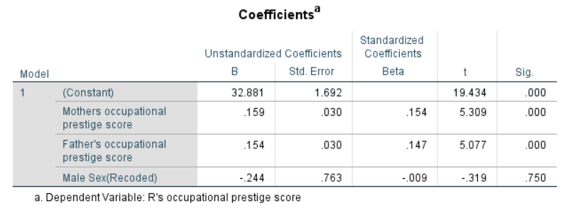
• The predicted occupational prestige score will increase by 0.159 for each unit increase of mother’s occupational prestige score, 0.154 for each unit increase of father’s occupational prestige score, and -0.244 for being male.
• The effects of moos on faos are statistically significant at the 0.001 level. The effect of sex (male) is not statistically significant.