Stata II
Inferential Statistics
After attending this training session, you will be able to:
- Get to know CITL and Stata
- Understand how to open data sets, set memory size
- Install user-written programs
- Learn about the General Social Survey (GSS)
- Obtain inferential statistics including chi-square test, t-test, ANOVA, bivariate correlation, linear regression, multiple regression
- Do practice exercises
- Print output
- Save and export output
Introduction
Code and Dataset
For this training session, please download the following data and code:
Recap of Stata I
In the Stata I training session, we covered the following topics. Please feel free to refer back to the Stata I workbook using the following links if you would like a refresher.
- What is Stata?
- Using the Data Editor
- Descriptive Statistics
- Data Transformation
- Graphics
- Saving and Printing
As in the Stata I training session, we will be using data from the General Social Survey.
Installing User-Written Programs in Stata
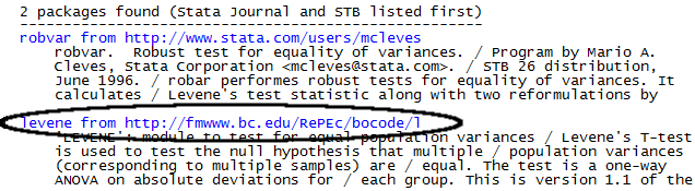
User-written programs can be installed by using the findit command. Your computer needs be connected to the Internet before submitting the findit statement. We will use this command to install the Levene’s test (levene), as this test will be used later in this tutorial but is not preinstalled in Stata. To search for this program, type:
findit leveneWhen the Viewer window opens, click on the link “levene from http://fmwww.bc.edu…”
To install levene, click on the link that says "(click here to install)"
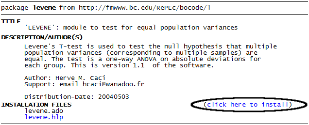
You will be directed to the screen below if installation was successful:

Chi-square test
A chi-square test is used to determine whether there is a statistically significant association between two categorical variables.
Example 1: 2x2 Table
Example 1 tests whether there is a significant association between the variables sex (Respondent’s sex) and the variable hschem (Respondent ever took chemistry class in high school). The syntax generates a crosstabulation table with chi-square test statistics. Enter:
tabulate sex hschem, all exactOutput:
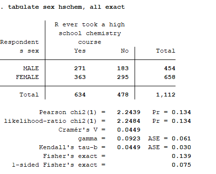
Stata generates the following test statistics for chi-square:
For all categorical variables:
- Pearson’s Chi-Square: Used to test the hypothesis that the row and column variables are independent. This should not be used if any cell has an expected value less than 1, or if more than 20% of the cells have expected values less than 5.
- Likelihood Ratio: A goodness-of-fit statistic similar to Pearson’s chi-square. This statistic is appropriate to report for smaller sample sizes. The likelihood ratio approaches the chi-square distribution as n increases, so for large sample sizes, the two statistics are the same and either can be reported.
- Cramér’s V: It shows the magnitude of negative or positive relationship between two variables which ranges from -1 to +1.
- Fisher’s Exact Test: A test for independence in a 2x2 table. This statistic is most useful when the total sample size and expected values are small.
- 1-sided Fisher’s Exact Test: The interpretation is the same as Fischer’s Exact Test except this result shows a p-value for 1-sided test.
For ordinal variables only: - gamma: This result is appropriate for ordinal variables because it uses the ordering within a variable to compute a test statistic. It is analogous to a correlation coefficient. The statistic ranges from -1 to +1. The gamma statistic will be close to zero when the relationship of two variables is independent. - Kendall’s tau-b: Similar to gamma, but makes a correction for pairs tied in the dependent variable - ASE: Asymptotic Standard Error, a standard error specifically computed for categorical (i.e. nominal and ordinal) data.
In this example, Fisher’s Exact Test indicates a p-value of .139. Thus, data like this are relatively consistent with the null hypothesis, and we can conclude that there is not a statistically significant relationship between the respondent’s sex and whether they took a chemistry course in high school.
Example 2: 3x2 Table
Example 2 tests whether is a significant association between the variables colsci (Respondents who took college-level science courses or not) and natspac (Attitudes towards the space exploration program). The syntax generates a crosstabulation table with chi-square test statistics. Enter:
tabulate colsci natspac, all expectedOutput:
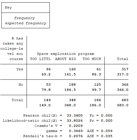
It is appropriate to use the Chi-Square test statistic in this example. For example, using Pearson Chi-Square, the level of significance is p < .05 level. Thus, there is a statistically significant relationship between attitudes towards the space program and taking college-level science courses.
Exercise 1
Perform a chi-square test to determine if educational attainment (degree) is significantly associated with the belief that marijuana should be legal (grass).
- How many high school graduates said “Yes” to legalization?
- Which chi-square test statistic is appropriate? Is there a statistically significant relationship between the two variables?
See Appendix A for answers.
Independent Samples t-test
An independent samples t-test determines whether there is a statistically significant difference in the mean of a continuous dependent variable between two groups.
For example, this procedure may be used to find out if there is a statistically significant difference between the responses of men and women (sex) for how much they have to relax per day (hrlax).
Before running an independent samples t-test, a test of the homogeneity of variance (Levene’s Test) must be conducted to determine whether the variances of the dependent variable hrlax between groups are equal or unequal. Enter:
levene hrlax, by (sex)Output:
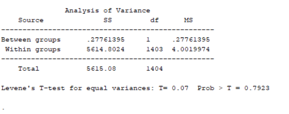 {fig-alt=“An analysis of variance for the Levene’s Test showing the results at the bottom where T=0.07 and Prob > T = 0.7923}
Because the p-value of Levene’s test is > 0.05, we fail to reject the null hypothesis and conclude that the two groups have equal variances. Therefore, the ttest syntax should not use the unequal option. Enter:
ttest hrlax, by(sex)Output:
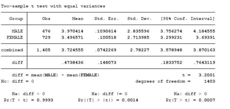
Because the t-test statistic significance level is 0.0014 (Ha:Diff!=0 for two tail) which is less than 0.05, we reject the null hypothesis and conclude that there is a statistically significant difference in hours have to relax per day between men and women.
Exercise 2
Find out if there is a statistically significant difference in terms of respondents’ family income (fmi) between respondents who took college-level science courses and those who did not?(colsci). See Appendix A for answers.
ANOVA
A one-way ANOVA is used to determine whether there is a statistically significant difference in the mean of a continuous dependent variable among two or more groups.
For example, this procedure may be used to test if there is a statistically significant difference in the average number of hours spent watching television per day (tvhours) by marital status (marital).
First, the levene command must be requested to determine if the equal variance assumption is met. (By default, the oneway command computes Bartlett’s Test for Equal Variances. However, we recommend Levene’s Test for Equality of Variances because it is relatively more robust to non-normality than other homogeneity tests.) Enter:
levene tvhours, by(marital)Output:
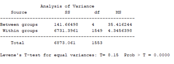
Because p < .05, as seen in the output table, we reject the null hypothesis that the variances are equal, and not-equal variances are assumed. The result confirms that we should use the Welch test for non-equal variances.
Note: Because of the result from Levene’s test above, we cannot perform a standard equal variance ANOVA test for these variables. If we want to use equal variance anova, we should use the code:
oneway tvhours marital, tabulateWelch Test
Because the homogeneity of variances assumption is not met, the Welch test of equality of means should be requested when performing a one-way ANOVA. To request the Welch test, wtest must be installed in Stata. Submit the below syntax and install “wtest from http://www.ats.ucla.edu…”:
findit wtest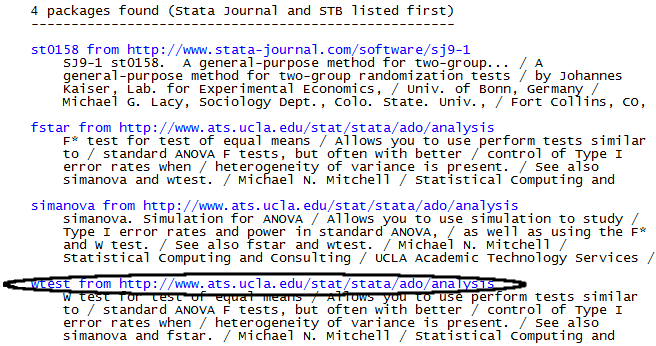
To perform the Welch test, enter:
wtest tvhours maritalOutput:

Because p < .05, we conclude tvhours significantly differs based on marital groups.
ANOVA Post Hoc Tests
Once you have determined that differences exist among the group means, post hoc tests can determine which means differ. Because the significance of the statistic found previously in levene tvhours, by(marital) was < .05, we reject the null hypothesis that the variances are equal. Therefore, we can select a post hoc test that assumes unequal variances.
Because the homogeneity of variances assumption is not met, the Games and Howell comparison of group means should be requested for post hoc. To request the Games and Howell test, pwmc must be installed in Stata. Submit the syntax below and install “pwmc from http://fmwww.bc.edu/…”:
findit pwmc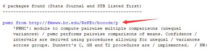
To perform the Games and Howell post hoc test, enter:
pwmc tvhours, over(marital)Output:
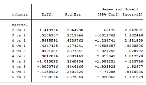
The Multiple Comparisons table provides the results of the Games and HoWell post hoc test. The values for the variable Marital: 1=Married, 2=Widowed, 3=Divorced, 4=Separated, 5=Never married. We use this confidence interval in the same way that we use a confidence interval for a regular independent samples t -test: if it contains 0.00, the groups are not significantly different, but if it does not contain 0.00 then the groups are significantly different.
From this table it can be concluded that:
- Group Married’s mean is significantly different from the group Widowed’s mean.
- Group Widowed’s mean is significantly different from group Never married’s mean.
- All the other groups based on marital status have no significant different with each other.
After identifying statistically significant differences, look back at the table of descriptive statistics to determine which marital groups spends more (or less) time watching TV per day. It is clear that the mean hours of time spent watching TV per day is significantly higher for group Widowed than othe groups.
For equal variance, The oneway command includes the capability of performing multiple-comparison tests, using either Bonferroni (bonferroni), Scheffé (scheffe), or Šidák (sidak) corrections. For example, if we use Bonferroni post hoc test for standard anonva with equal variance of homogeneity, we should enter :
oneway tvhours age, noanova bonferroniExercise 3
Using the one-way ANOVA procedure, test whether respondents’ family income (fmi) is different based on respondents’ education level (degree). See Appendix A for answers.
Bivariate Correlation
A (bivariate) correlation coefficient measures the linear relationship between two continuous variables. A correlation coefficient ranges from -1 to 1. A positive correlation coefficient indicates that there is a positive linear relationship, whereas a negative correlation coefficient indicates that there is a negative linear relationship. A correlation coefficient of 0 indicates that there is no linear relationship between two variables.
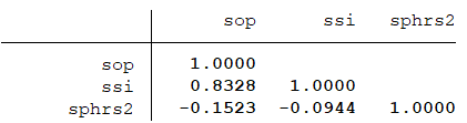
For example, this procedure may be used to measure the relationship between the continuous variables spouse occupation prestige score (sop), spouse socioeconomic index score (ssi), and number of hrs spouse usually works a week (sphrs2). Enter:
pwcorr sop ssi sphrs2, obs sig star(0.05)Output:
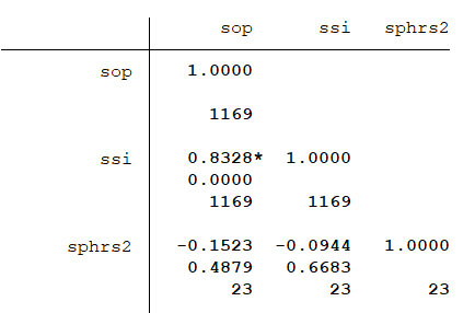
The output is a 3x3 table. Each cell contains (1) the correlation coefficient (Pearson Correlation), (2) the p-value associated with the correlation coefficient (Sig.), and (3) the number of cases (N). In this example, the correlation coefficient between sop and ssi is 0.8328. and the significance of the coefficient is reported as 0.0000, which suggests that these two variables are positively correlated at 0.05 level.
Note on sample size (N): The third row of the cells for the correlation of sphrs2 and sop, and sphrs2 and ssi show that only 23 cases are used for computation for both pairs. Meanwhile, the correlation of ssi and sop used 1,169 cases.
The default treatment of missing cases is to use the maximum number of non-missing values for each pair of variables, which is known as pairwise deletion. The pwcorr command uses pairwise deletion.
An alternative treatment of missing cases is listwise deletion. The correlate command calculates a correlation coefficient using listwise deletion, which omits all cases with at least one missing value in all given variables. When only two variables are included, the sample size is the same whether pairwise or listwise deletion is used. However, these options make a difference in the sample size when three or more variables are included. Enter:
correlate sop ssi sphrs2Output:
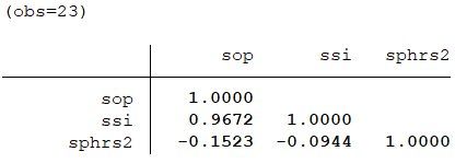
To compare enter:
pwcorr sop ssi sphrs2Output:
Exercise 4
Compute the correlation between: the highest year of school completed (educ), the respondent’s father’s occupational prestige index (faos), and the respondent’s mother’s occupational prestige index (moos) using (1) pairwise deletion and (2) listwise deletion and compare how the sample size changes. See Appendix A for answers.
Bivariate Regression
Bivariate linear regression is used to model the effect of a numeric independent variable on a numeric dependent variable.
This example uses linear regression to measure the effect of educational attainment (educ) on respondent’s income (realrinc). In Stata, the regress command estimates a linear regression model with the dependent variable listed first and the independent variable(s) listed second. Enter:
regress realrinc educOutput:
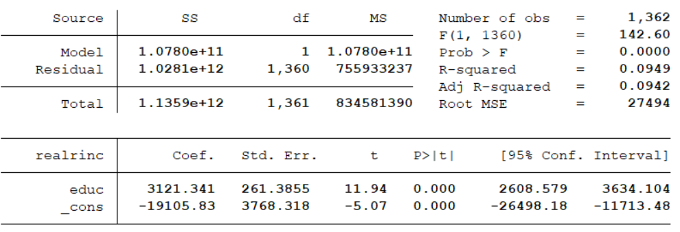
The ANOVA table (upper left, box 1) tests whether the independent variable (educ) has a linear relationship with the dependent variable (realrinc). The ANOVA F-score (box 2, upper right) is statistically significant, F(1, 1362) = 142.60, Sig = 0.0000, thus the education variable has a significant linear relationship with the income variable.
We can also use the information in box 2 to assess the overall fit of the model. R-squared, also called the coefficient of determination, tells us the proportion of all variation in the dependent variable that is explained by the independent variable. The R-squared ranges ranges from 0 (no effect of an independent variable on a dependent variable) to 1 (perfect prediction of the dependent variable by the independent variable). From box 2, we see that 9.49% of the variation in income (dependent variable) is explained by the years of education (independent variable).
The adjusted R-squared is used for model selection and is adjusted for the number of independent variables in the model.
Box 3 (lower) presents the unstandardized regression coefficients, their standard errors, t-statistics, significance levels, and the 95% confidence intervals for the coefficients. The regression coefficient for the constant is -19105.83 and the gregression coefficient for educ is 3121.341. We can use these values to express the linear regression equation: Y = -19105.83 + 3121.341(educ). The slope, 3121.341 is called an unstandardized coefficient because the effect is measured in the original scale of the variable. In this example with a one unit increase in the years of education, predicted income will increase by $3,121.341.
The standard error (Std.Err.) is used to calculate the t-value (coefficient/Std. Error). This is the test statistic for the significance test where the null hypothesis states that the unstandardized coefficient is equal to 0. In this example, the coefficient for educ is statistically significant. This means that you can reject the null hypothesis that the education variable’s coefficient is equal to 0 and conclude that education is a significant predictor of income.
Exercise 5
Run a bivariate linear regression to assess the effect of respondent’s age (age) on their performance of the vocabulary test score (wordsum). See Appendix A for answers.
Multiple Regression
Multiple regression is the same as bivariate regression, except it uses two or more independent variables to explain the variation of the dependent variable. This example uses Multiple regression to measure the effect of respondents’ health score (rhs) and age (age) on respondent’s income (realrinc). The beta option requests standardized regression coefficients. Enter:
regress realrinc rhs age, betaOutput:
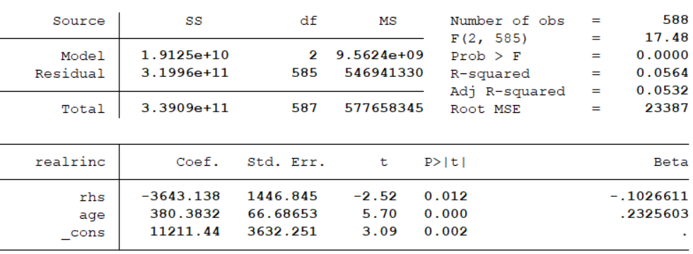
The top left hand side shows the results of the ANOVA tests. The ANOVA tests examines whether the independent variables (rhs and age) have a linear relationship with the dependent variable (realrinc). In this example, the ANOVA F-score is statistically significant, F = 17.48, Sig = 0.0000; thus a respondent’s health score and age have a significant linear relationship with income.
The introduction of additional variables to a model produces a higher R-squared value, regardless of the efficiency of the model. Thus, R-squared as a model selection tool always favors models with additional predictors.
The Adjusted R-Squared value corrects this bias by adjusting both the numerator and the denominator of the R-Squared by their respective degrees of freedom. The adjusted R-squared is calculated using the equation below, where n is the number of observations and k is the number of independent variables.
\[ \text{Adjusted R-Squared } = 1-(1-R)^2 * \frac{(n-1)}{(n-k-1)} \]
Unlike R-squared, the Adjusted R-squared can decline in value as more predictors are added. It is important to keep in mind, however, that the R-Squared value is a proportion of total variance, while the Adjusted R-Squared is not.
The Coefficients table provides the values of unstandardized regression coefficients (B), standardized coefficients (Beta), t-test statistics (t), and p-values (Sig.).
- The value of unstandardized regression coefficient shows that a unit increase in rhs (worse health condition) will decrease predicted income by $3643.138 while holding age as constant.
- The t-test statistic is -2.52, and the p-value associated with the t-test statistic is 0.012. This results show that rhs is statistically significant at the 0.05 level while controlling for age.
The standardized coefficient (Beta) measures change in the dependent variable in standard deviations per one standard deviation change in the independent variable. The purpose of using standardized coefficients is to compare the magnitude of the effect of each independent variable. Because the absolute value of standardized coefficient for age is larger than that for rhs, we can conclude that age has a larger impact on real income than health rating.
Exercise 6
Run multiple regression to assess the effect of occupational prestige of a respondent’s parents (faos and moos) and respondent’s gender (Male) on the respondent’s occupational prestige (pres). See Appendix A for answers.
Appendix A: Answers for Exercises
Exercise 1
Enter:
tabulate grass degree, all expected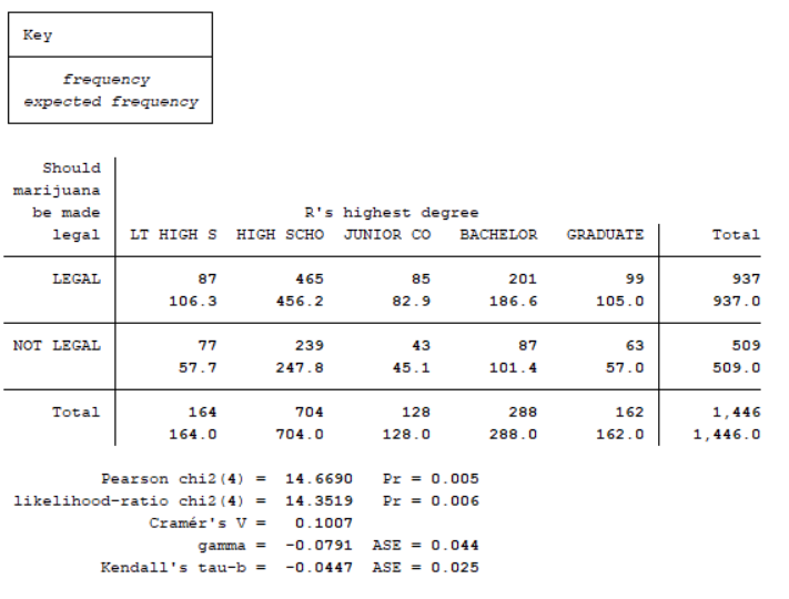
- 465 high school graduates said ``Yes’’ to legalization.
- Because the expected cell counts are greater than five, Pearson’s chi-square test is appropriate. Because the p-value associated with the Pearson chi-square statistic (0.005) is less than 0.05, there is a statistically significant relationship between the two variables.
Exercise 2
Enter:
levene fmi, by(colsci)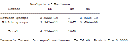
Because the Levene’s Test for Equality of Variances is significant (p < 0.05), the “unequal” option is necessary.
Enter:
ttest fmi, by(colsci) unequal\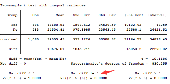
The P statistic (.0000) is significant (p < 0.05), therefore the amount of respondent’s family income respondents made significantly differ based on if they took or didn’t take college-level science courses.
Exercise 3
Enter:
levene fmi, by(degree)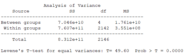
We use the similar levene test step as we did in Exercise 2. Because the Levene’s Test is significant (p < .05), we reject the homogeneity of variance assumption. Thus, we can conduct a unequal variance for ANOVA using Welch test. Enter:
wtest fmi degree
Because p < .05, we conclude that differences in average income among educational groups are statistically significant.
We now explore the nature of those differences using Games and Howell post hoc tests. Enter:
pwmc fmi, over(degree)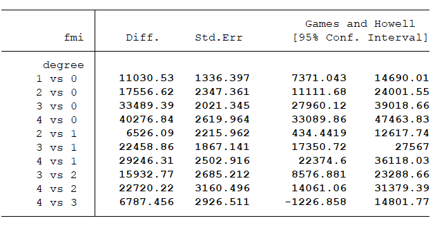
The Multiple Comparisons table provides the results of the Games and Howell post hoc test. The values for the variable degree: 0=Less than High School, 1=High School, 2=Junior College, 3=Bachelor, 4=Graduate.
To decide significance:if confidence interval contains 0.00, the groups are not significantly different, but if it does not contain 0.00 then the groups are significantly different.
- Group Less than High School is significantly different from all other groups at 0.05 level.
- Group High School is significantly different from all other groups at 0.05 level.
- Group Junior college is significantly different from all other groups at 0.05 level.
- Group Bachelor is significantly different from all other groups except group Graduate(and vice versa).
Exercise 4
Correlation with Pairwise Deletion. Enter:
pwcorr educ faos moos, obs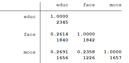
Correlation with Listwise Deletion. Enter:
correlate educ faos moos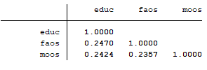
Educational attainment (educ) is positively correlated with mother’s (moos) and father’s (faos) occupational prestige score index (PSI). Mother’s and father’s PSI are also positively correlated. The direction of the relationship does not change much if you use either pairwise or listwise deletion. The strength of the relationship does change slightly depending on the treatment of missing cases.
Exercise 5
Enter:
regress wordsum age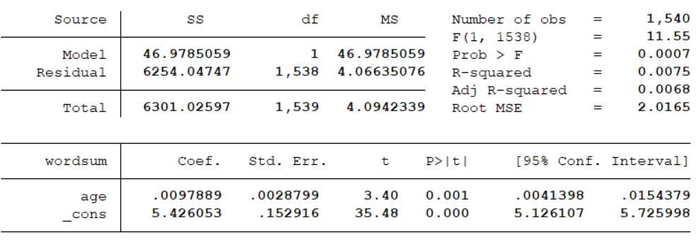
- 0.75% of the variation in vocabulary test score is explained by age.
- Because the F-statistic is statistically significant, age has a significant positive prediction with vocabulary test score.
- The regression coefficient for the constant is 5.426 and the coefficient for the independent variable age is 0.01. The predicted vocabulary test score will increase by 0.01 for each additional year of age.
- The effect of age on wordsum is statistically significant at the 0.01 level.
Exercise 6
Enter:
regress pres moos faos Male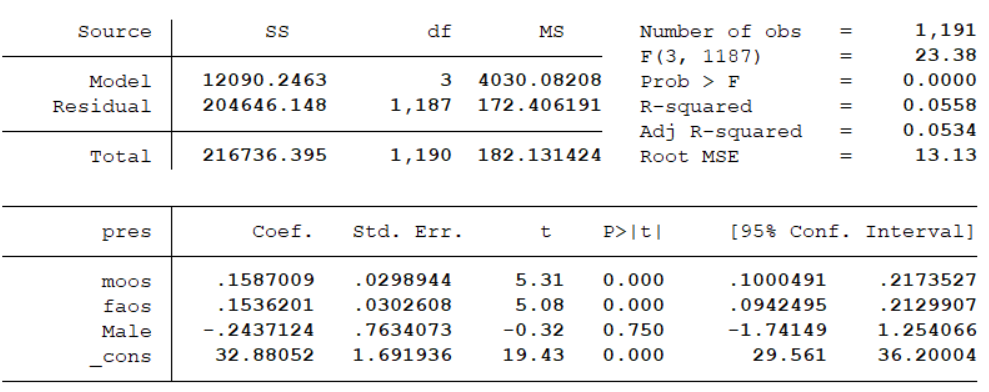
- 5.58% of the variation in the respondent’s occupational prestige is explained by the variables in this model.
- Because the F-statistic is statistically significant, at least one independent variable of mother’s occupational prestige score, father’s occupational prestige score, and gender is a significant predictor of the respondent’s occupational prestige score.
- The predicted occupational prestige score will increase by 0.1587 for each unit increase of mother’s occupational prestige score, 0.1536 for each unit increase of father’s occupational prestige score, and -0.244 for being males.
- The effects of faos and moos are statistically significant at the 0.001 level. The effect of gender (male) is not statistically significant.