Python II

Intermediate Python

This notebook contains content for the Python II training session. We will cover the following topics:

Working With DataFrames: Data transformation
Inferential Statistics
Visualizations
Saving and exporting
Advanced Topics and Examples
Common external libraries and frameworks across various domains

Important

This training session is conducted on Google Colab. The instructions below assume that you are viewing this notebook directly on Colab.

If you wish to use this notebook locally, ensure that you are running at least Python 3.11 and all the necessary package dependencies are met. You can skip some of the setup code cells that are marked “Colab Only” at the beginning of the cell. You may also need to modify the path to the dataset file to the appropriate location on your local machine.

Introduction

Jupyter Notebooks

Earlier called the IPython notebook (hence the .ipynb extension), Jupyter notebooks are an open-source web application that allows you to create and share documents that contain live code, equations, visualizations, and narrative text. They are widely used for data cleaning and transformation, numerical simulation, statistical modeling, data visualization, machine learning, etc.

Google Colaboratory (Colab in short) is built on top of Jupyter notebooks and has added functionalities that are found in more conventional IDEs like PyCharm, RStudio, Spyder, etc.

Colab is entirely cloud-based and the free tier even allows for some free GPU and TPU processing capabilities. Additionally, it can connect with your Google Drive storage for accessing and storing data.

In case you want to install Python and Jupyter notebooks on your local machine, we recommend you follow this guide to install Anaconda. Anaconda is a popular tool that installs and manages Python on your system, which can help prevent package conflicts as you install more Python libraries in the future.

Common shortcuts

Jupyter Notebook cells have 2 modes, ‘Command’ and ‘Edit’.

To switch from command to edit mode press Enter. To switch from edit to command mode press Esc.

Execute cell: Ctrl+Enter Execute cell and move to next cell: Shift+Enter (This will add a new cell below if none exists) Execute cell and add new cell below: Alt+Enter

In command mode: - insert cell above: a - insert cell below: b - change cell type to Markdown: m (Ctrl+mm in Colab) - change cell type to code: y (Ctrl+my in Colab) - delete cell: dd (Ctrl+md in Colab)

Setup

Run the cell below to mount your Google Drive folder and create a copy of the training materials. You will need to provide permission to Colab for accessing your Drive.

from google.colab import drive
drive.mount('/gdrive', force_remount=True)

Magic Commands

Jupyter notebooks allow you to execute certain operations outside of the Python environment. Often, we might need to directly access the system terminal for installing new packages and make other changes outside the environment. These are called magic commands and begin with !.

You can even turn an entire cell to access an outside environment by specifying it with the %% in the first line. Every subsequent command within the cell will refer to the external environment and not Python (without using !). Here, we are going to use the bash shell to download the dataset used for this workshop and save it in your Drive folder.

### Colab only###

%%bash
mkdir /gdrive/MyDrive/Colab\ Notebooks/pyworkshop # Creates new folder called pyworkshop
ls /gdrive/MyDrive/Colab\ Notebooks/ -l # Check if the new folder was created

Download a copy of the dataset file used for this training session.

import requests
import os

url = 'https://raw.githubusercontent.com/citl-data/training_session_data/main/GSS2018.csv'
target_dir = '/gdrive/MyDrive/Colab Notebooks/pyworkshop' # Modify path if runnning locally
file_path = os.path.join(target_dir, 'GSS2018.csv')

response = requests.get(url)
with open(file_path, 'wb') as f:
    f.write(response.content)

Working With DataFrames: Data transformation

A majority of data analysis in Python will involve using the pandas library to deal with dataframes. It provides similar functionalities to R dataframes.

Let’s first import the GSS 2018 data.

import pandas as pd
my_data = pd.read_csv('/gdrive/MyDrive/Colab Notebooks/pyworkshop/GSS2018.csv')

While working with data sets, we often need to create new variables or recode the current variable into new values. This can also be easily done with the help of pandas.

Creating a new variable

To create a new variable in Python, you can directly use varname = to specify this new variable.

But to create a new variable in a dataframe, you have to use the object name and the dataframe to specify the name of the created variable.

For instance, you need to type my_data['birth_year'] = rather than 'birth_year' = so that the system understands the newly created variable is an element of my_data rather than a stand-alone variable.

Let’s compute people’s birth_year based on their age.

my_data['birth_year'] = 2018 - my_data['age']

# use describe() to see the descriptive statistics
my_data['birth_year'].describe()

You can also check whether the new variable has been created successfully by previewing the dataframe.

# Display all the columns
pd.set_option('display.max_columns', None)

my_data.head()

Recoding variables

Recoding variables with pandas is simple.

The recode procedure transforms an existing variable into a new variable by changing, rearranging, or consolidating the values of the existing variable. It allows the user to:

Change an existing categorical variable into a new categorical variable with a smaller number of categories/levels.
Change an existing continuous variable with many unique values (e.g, income, age, etc.) into a categorical variable with fewer levels (for example, if recoded, the variable income will have the values low, medium, and high, while the variable age will have young, adult, and senior as values).
Code missing values.
Replace miscoded values with correct values.
Create a dummy variable based on a cutoff value.

To recode a variable, one or more of Python’s logical operators are used. You may refer to our Python I Notebook for common logical operators.

For instance, if you want to recode age based on the following rule:

age <= 21: non-adult;
age > 21: adult

You can use the np.where function:

import numpy as np
my_data['age_group'] = np.where(my_data['age'] > 21, "adult", 'non-adult')

# You can use value_counts() to get the frequency of each value
my_data['age_group'].value_counts()

If the original variable is categorical, we can use replace function to recode the values.

For example, let’s check the variable ‘sex’. Let’s recode it using the following rule:

1 –> 'Male'
2 –> 'Female'

my_data['sex'].value_counts()

my_data['sex'] = my_data['sex'].replace({1:"Male", 2:"Female"})

my_data['sex'].value_counts()

Exercise 1

Recode marital using the following rule:

1: 'MARRIED', 2: 'WIDOWED', 3: 'DIVORCED', 4: 'SEPARATED', 5: 'NEVER MARRIED', 9: np.nan

# Note: notice how we recode 9 into missing values here

# Use isna() to detect where a value is missing and then sum() to get total number of missing values in the column
my_data['marital_labeled'].isna().sum()

Inferential Statistics

!pip install -q pingouin

import pingouin as pg
import scipy.stats as stats

Contingency table and chi-square test

The crosstab() function creates a contingency table.

A contingency table is used to show the joint distribution of cases over two or more categorical variables. The basic syntax to produce a contingency table,mytab = pd.crosstab(var1, var2), will result in a table with var1 in the rows and var2 in the columns.

Let’s create a contingency table using the variables marital_labeled and sex.

# Contingency table
# A contingency table is used to show the joint...
# ...distribution of cases over two or more categorical variables.
# The basic syntax to produce a contingency table is
# mytab = pd.crosstab(var1 (index), var2 (columns))
# For example, var1 = marital and var2 = sex

mytable = pd.crosstab(my_data["sex"], my_data["marital_labeled"])
mytable

If you wish to see the percentage, you can do it by specifying the value of normalize to index or column or all.

# To see the percentage
mytable_percentage = pd.crosstab(my_data["sex"], my_data["marital_labeled"], normalize = 'all')
mytable_percentage

If you would like to run statistical tests and analyses like Pearson’s χ2 test on the two variables, we can use the chi2_independence function from the pingouin library.

expected, observed, stat_vals = pg.chi2_independence(my_data, x='sex', y='marital_labeled')
stat_vals
# print(f'Expected values: {expected}')
# print(f'Observed values: {observed}')

Exercise 2

Find out if there is a significant association between country of birth born and speaking a language other than English othlang.

# Your code here
# Step 1: perform test


# Step 2: interpret the result

Independent samples t-test

An independent samples t-test determines whether there is a significant difference in the means of a continuous variable between two groups.

For this example, we’ll test whether there is a significant difference in the responses between men and women sex and how much time they have to relax per day hrlax

Before performing a t-test, we need to compare the variances of two samples. Different t-test methods make different assumptions about whether or not the variances of the two samples differ. To test for equality of variances, we will perform a Levene’s Test using the stats.levene function of the scipy library.

lev, p = stats.levene(my_data[my_data['sex']=='Male']['hrlax'],
                my_data[my_data['sex']=='Female']['hrlax'], nan_policy='omit')
# Notice that we include an addiitonal argument to handle missing data

print(f'The p-value of the Levene test is {p}')

The Levene method tests the null hypothesis that the variances are equal. Because the significance of Levene’s test in this example is larger than 0.05, we fail to reject the null hypothesis, and the assumption of equal variance is met. In such a case, the statistics for equal variances assumed should be used.

We’ll use the pg.ttest function to test whether there is a significant difference in means between the two groups. Notice that it includes a parameter called correction. It is recommended to set it to auto, which will automatically use Welch T-test when the equal variances assumption is violated.

# Running an independent samples t-test

pg.ttest(my_data[my_data['sex']=='Male']['hrlax'],
         my_data[my_data['sex']=='Female']['hrlax'],
         correction='auto')

Exercise 3

Compare average income of male and female using the variable sex_new and realrinc and interpret the result.

# your code here

# step 1: get the mean of realrinc for both female and male separately



# step 2: perform t test



# step 3: interpret the result

ANOVA

A one-way ANOVA (analysis of variance) is used to determine whether there is a statistically significant difference in the mean of a continuous dependent variable among more than two groups.

For this example, we’ll test whether there is a significant difference in means in the hours spent watching TV tvhours between different marital statuses marital_labeled.

We will again need to test for equality of variances among groups using the stats.levene function.

We can then use either pg.anova or pg.welch_anova functions.

lev, p = stats.levene(my_data[my_data['marital_labeled']=='MARRIED']['tvhours'],
                      my_data[my_data['marital_labeled']=='WIDOWED']['tvhours'],
                      my_data[my_data['marital_labeled']=='DIVORCED']['tvhours'],
                      my_data[my_data['marital_labeled']=='SEPARATED']['tvhours'],
                      my_data[my_data['marital_labeled']=='NEVER MARRIED']['tvhours'],
                      nan_policy='omit')

print(f'The p-value of the Levene test is {p}')

# Conducting a one-way ANOVA

# If the Levene's test was not significant, that is, equal variances are assumed:

aov = pg.anova(data=my_data, dv='tvhours', between='marital_labeled')
print('One-way ANOVA\n',aov)


# If the Levene's test was significant, that is, equal variances are not assumed:

welchaov = pg.welch_anova(data=my_data, dv='tvhours', between='marital_labeled')
print('\n Welch ANOVA\n',welchaov)

While the ANOVA procedure determines whether differences exist among the group means, post hoc tests are needed to determine which means differ from one another. Which post hoc test you use depends on the homogeneity of the variances.

# Conducting post-hoc tests

# Tukey's HSD

# pg.pairwise_tukey(data=my_data, dv='tvhours', between='marital_labeled').round(3)

# Games-Howell test

pg.pairwise_gameshowell(data=my_data, dv='tvhours', between='marital_labeled').round(3)

Exercise 4

Test whether the income differs significantly among different education levels using the variable degree and realrinc.

Then perform ANOVA test and interpret the result

# your code here


# step 1: conduct Levene's test



# step 2: perform ANOVA



# step 3: interpret the result

Correlation Matrix

Correlation is a measure of the linear relationship between two continuous variables. A correlation coefficient ranges from -1 to 1. A positive correlation coefficient indicates a positive linear relationship (i.e., as one variable increases, the other tends to as well). On the other hand, a negative correlation coefficient indicates a negative linear relationship. A correlation coefficient of 0 indicates there is no linear relationship between the two variables.

# Get the correlation matrix between age, realinc, hrs1, and tvhours

my_data[['age','realrinc','hrs1','tvhours']].corr()

# Correlation matrix with significance levels

my_data[['age','realrinc','hrs1','tvhours']].rcorr()

Linear Regression

Linear regression is used to assess the association between one or more independent variables (continuous or categorical) and a continuous dependent variable.

We’ll use the pg.linear_regression function to fit a linear regression model to test the association between the family income realrinc and other independent variables.

# Simple or bivariate regression with age as the only IV

lm1 = pg.linear_regression(my_data['age'], my_data['realrinc'], remove_na=True)
lm1

# Multiple linear regression with age and occupational prestige score as IVs

lm2 = pg.linear_regression(my_data[['age','pres']], my_data['realrinc'], remove_na=True)
lm2

Visualizations

Histogram

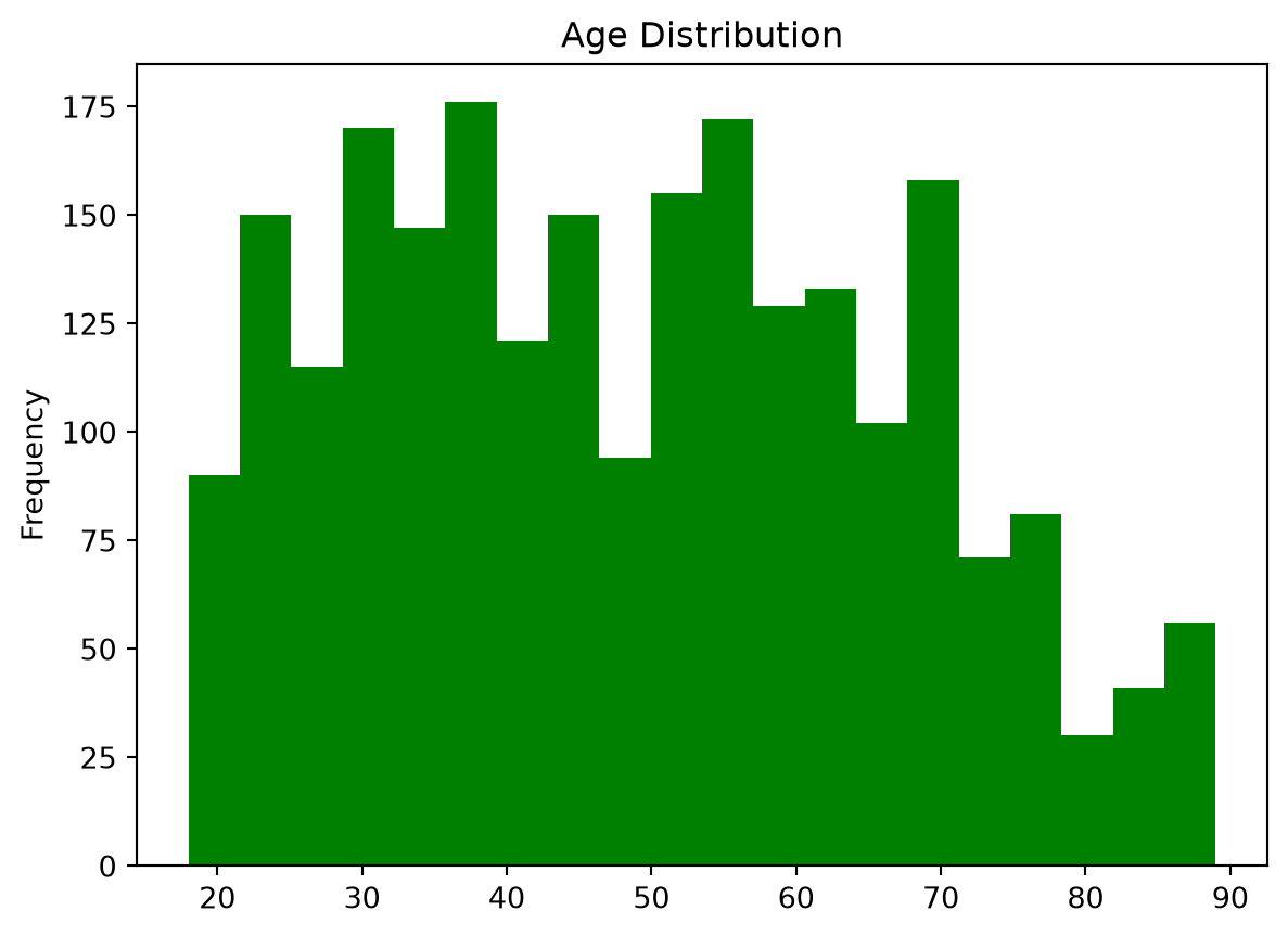
A histogram visually displays the distribution of a continuous variable. In Python, the plot.hist function works as shown below.

# Graphics
# Histogram
my_data['age'].plot.hist(title = 'Age Distribution',
                         color = 'green',
                         bins = 20)

Bar graphs

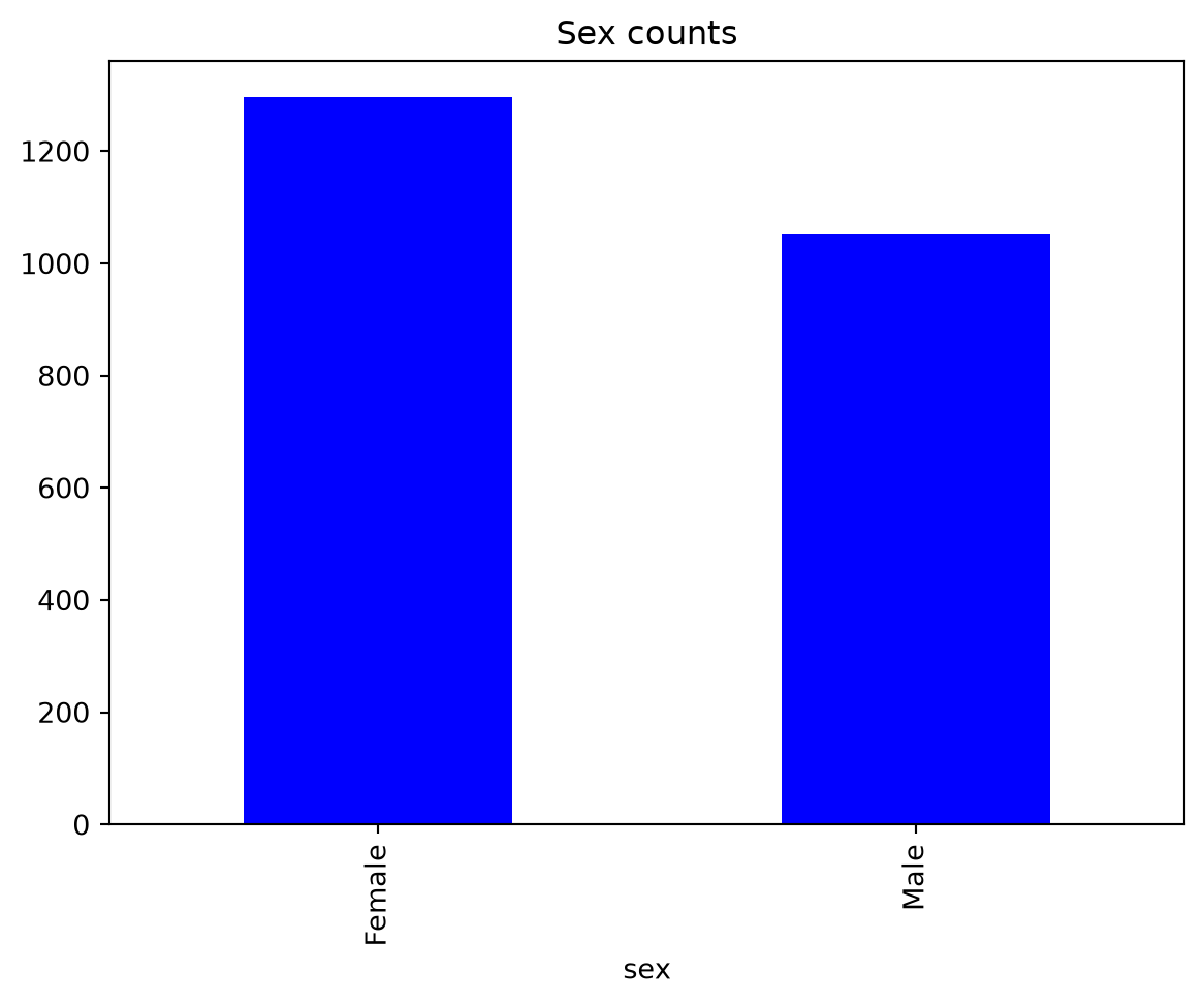
A bar graph can display the frequencies or distribution of a categorical variable. First, a data table must be created for plotting. In this case, we name our data table sexcount, then plot the bar graph of the sex variable by using the plot.bar function.

# Bar Graph
sexcount = my_data['sex'].value_counts()
sexcount.plot.bar(title = 'Sex counts',
                 color = 'blue')

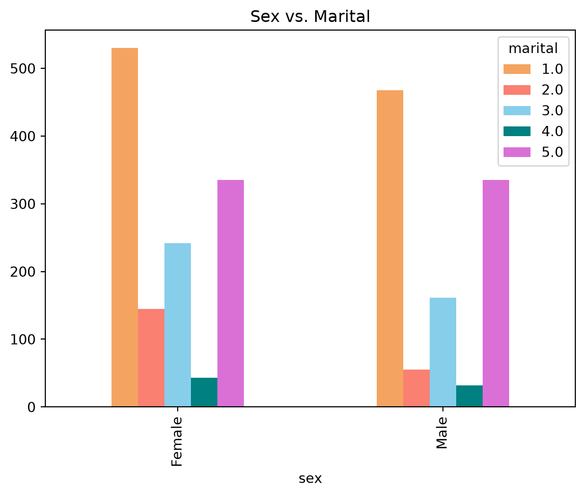
A grouped bar graph is a bar graph that uses an additional variable to group the plotted data. For example, you can create a grouped bar graph displaying sex and marital status. If you would like to plot the grouped bar plot of sex and marital variables, you will need to first use the crosstab command to get the frequencies and then use the plot.bar function.

# Grounded bar graph
groupbar = pd.crosstab(my_data['sex'], my_data['marital'])

groupbar.plot.bar(title = 'Sex vs. Marital',
                 color = ['sandybrown','salmon','skyblue','teal','orchid','cornflowerblue'])


# Named colors https://matplotlib.org/stable/gallery/color/named_colors.html

Exercise 5

Create a grouped bar chart to show the number of respondents across the variable degree and sex. The x is degree, y is the frequency and the group is sex

# your code here

# step 1: get the crosstable



# step 2: plot the grouped bar chart

Scatterplot

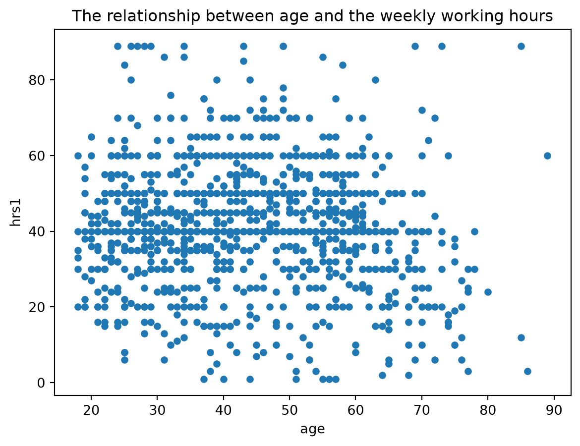
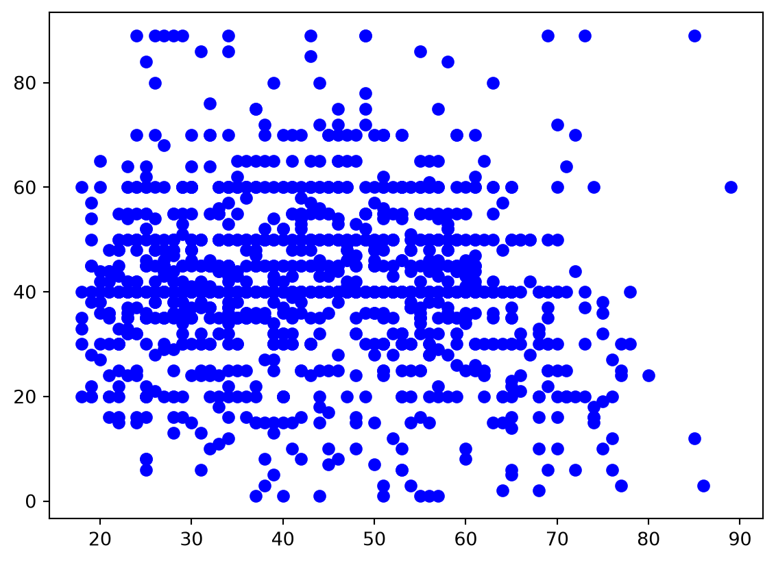
A scatterplot plots the “positions” of two variables in dimensions x and y. Let’s plot the the relationship between age and weekly working hours.

# Scatterplot
my_data.plot.scatter(x = 'age', y = 'hrs1',
                     title = 'The relationship between age and the weekly working hours')

Using Matplotlib library for advanced visualizations

When it comes to more complex visualizations, or when you want to customize your plots, you can use the Matplotlib library. Matplotlib is a comprehensive library for creating static, animated, and interactive plots in Python. It is a powerful library that can be used to create a wide range of plots, including histograms, scatter plots, bar charts, pie charts, and more.

import matplotlib.pyplot as plt

Scatterplot

# create a scatter plot where x being age and y being hrs1
plt.scatter(my_data['age'], my_data['hrs1'], color = 'blue')

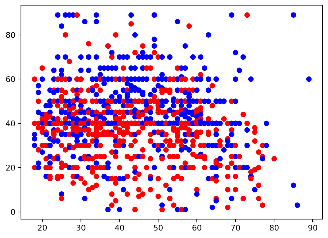
# create a scatter plot where x being age and y being hrs1, also differentiating the color by gender
colors = {'Male': 'blue', 'Female': 'red'}

plt.scatter(my_data['age'], my_data['hrs1'],
            c=my_data['sex'].map(colors), label=my_data['sex'])

Line chart

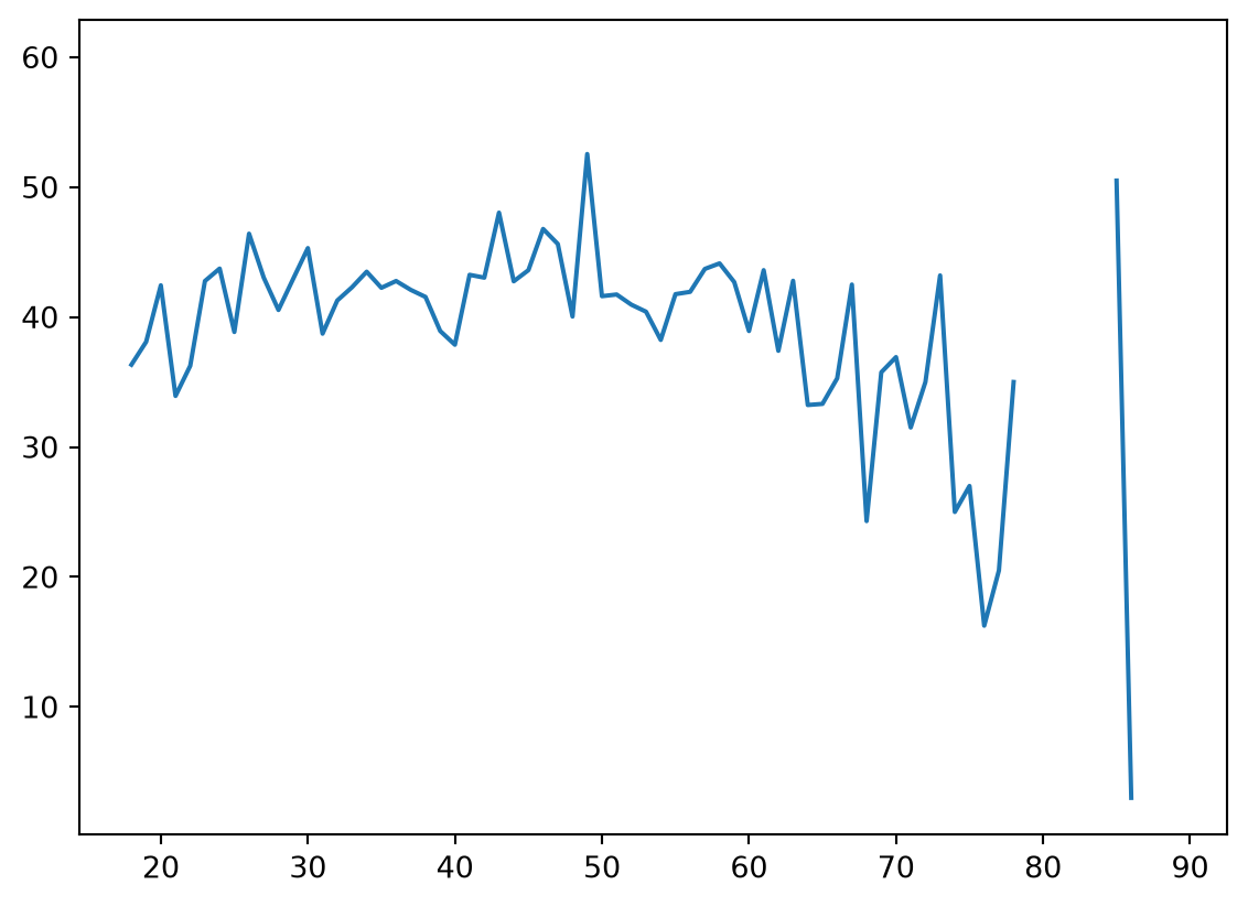
# group by age and calculate the mean of hrs1 and mean of sphrs1
hr_by_age = my_data.groupby('age').agg({'hrs1':'mean'}).reset_index()

plt.plot(hr_by_age['age'], hr_by_age['hrs1'])
plt.show()

Multiple charts

hr_by_age = my_data.groupby('age').agg({'hrs1':'mean','sphrs1':'mean'}).reset_index()
hr_by_age = hr_by_age[hr_by_age['age'] != 99]

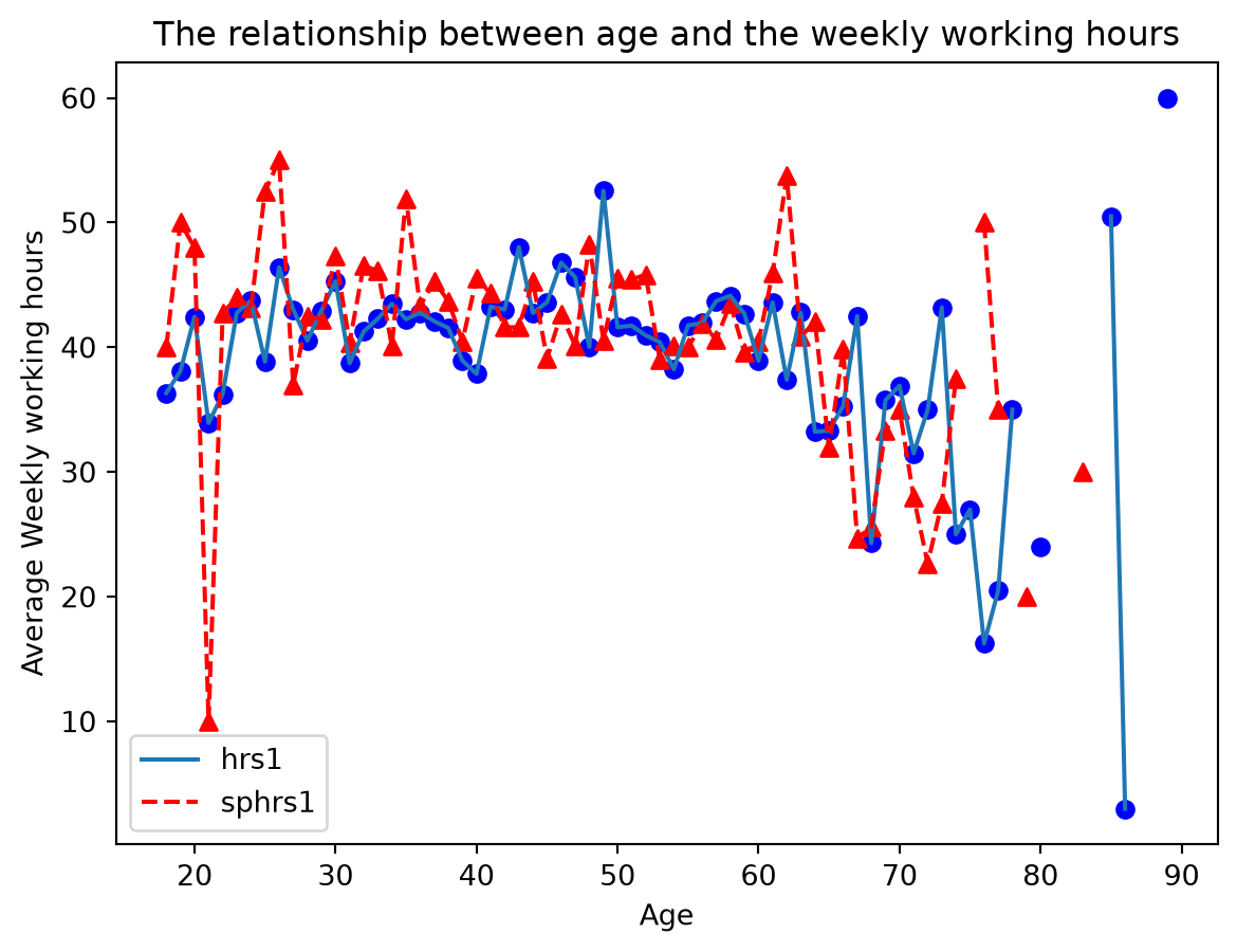
plt.plot(hr_by_age['age'], hr_by_age['hrs1'], label = 'hrs1')
# add title
plt.title('The relationship between age and the weekly working hours')
# add x and y axis labels
plt.xlabel('Age')
plt.ylabel('Average Weekly working hours')
# add points
plt.scatter(hr_by_age['age'], hr_by_age['hrs1'], color = 'blue')
# add a new line for sphrs1 using dotted line
plt.plot(hr_by_age['age'], hr_by_age['sphrs1'], label = 'sphrs1', color = 'red', linestyle = '--')
# add points for sphrs1 using a different triangle marker
plt.scatter(hr_by_age['age'], hr_by_age['sphrs1'], color = 'red', marker = '^')
# add legend by color
plt.legend()
plt.show()

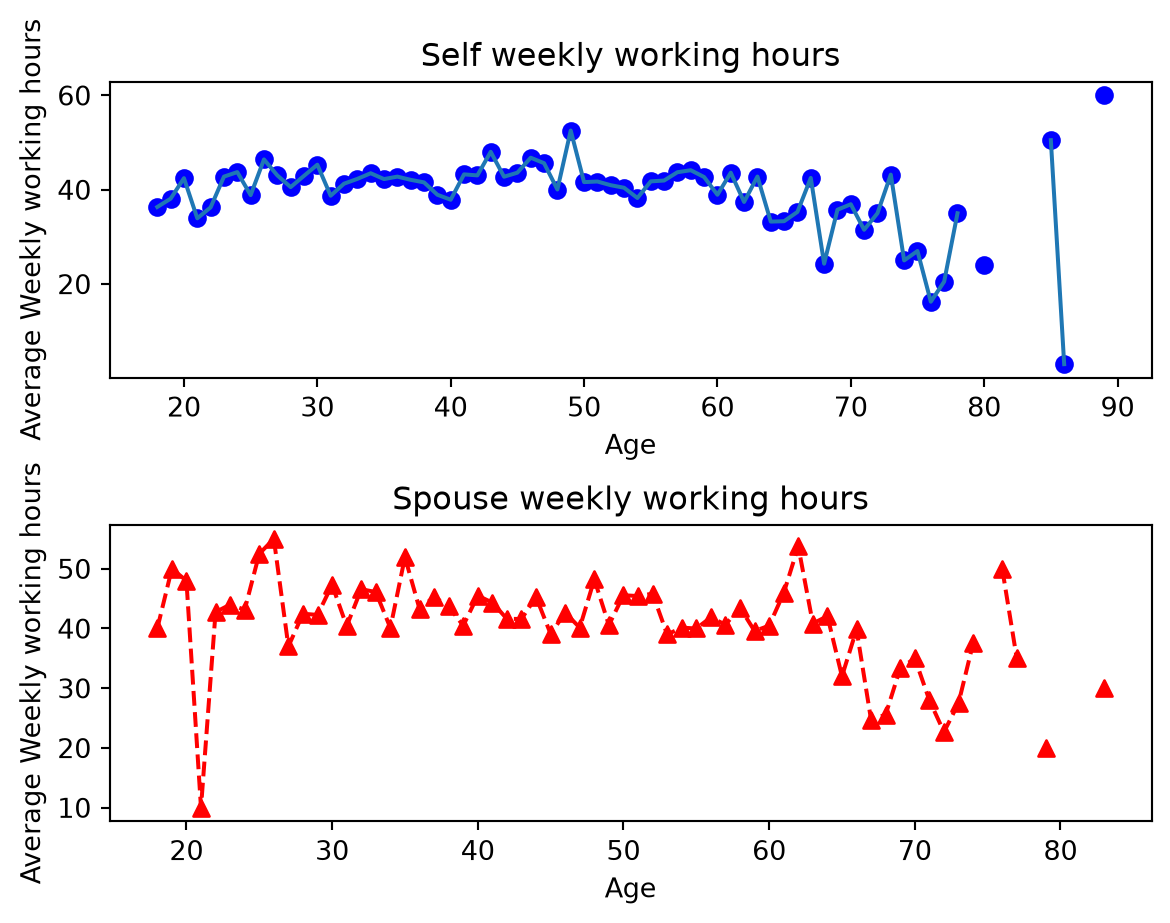
plt.figure()
plt.subplot(211) # plt.subplot(nmk) where n is the number of rows, m is the number of columns, and k is the plot number
plt.plot(hr_by_age['age'], hr_by_age['hrs1'], label = 'hrs1')
# add title
plt.title('Self weekly working hours')
# add x and y axis labels
plt.xlabel('Age')
plt.ylabel('Average Weekly working hours')
# add points
plt.scatter(hr_by_age['age'], hr_by_age['hrs1'], color = 'blue')
# add some blank space between the two plots
plt.subplots_adjust(hspace = 0.5)

plt.subplot(212)
plt.plot(hr_by_age['age'], hr_by_age['sphrs1'], label = 'sphrs1', color = 'red', linestyle = '--')
plt.title('Spouse weekly working hours')
# add x and y axis labels
plt.xlabel('Age')
plt.ylabel('Average Weekly working hours')
# add points for sphrs1 using a different triangle marker
plt.scatter(hr_by_age['age'], hr_by_age['sphrs1'], color = 'red', marker = '^')
plt.show()

income_by_age_gender = my_data.groupby(['age','sex']).agg({'realrinc':'mean'}).reset_index()
income_by_age_gender

income_by_age_male = income_by_age_gender[income_by_age_gender['sex'] == 'Male']
income_by_age_female = income_by_age_gender[income_by_age_gender['sex'] == 'Female']

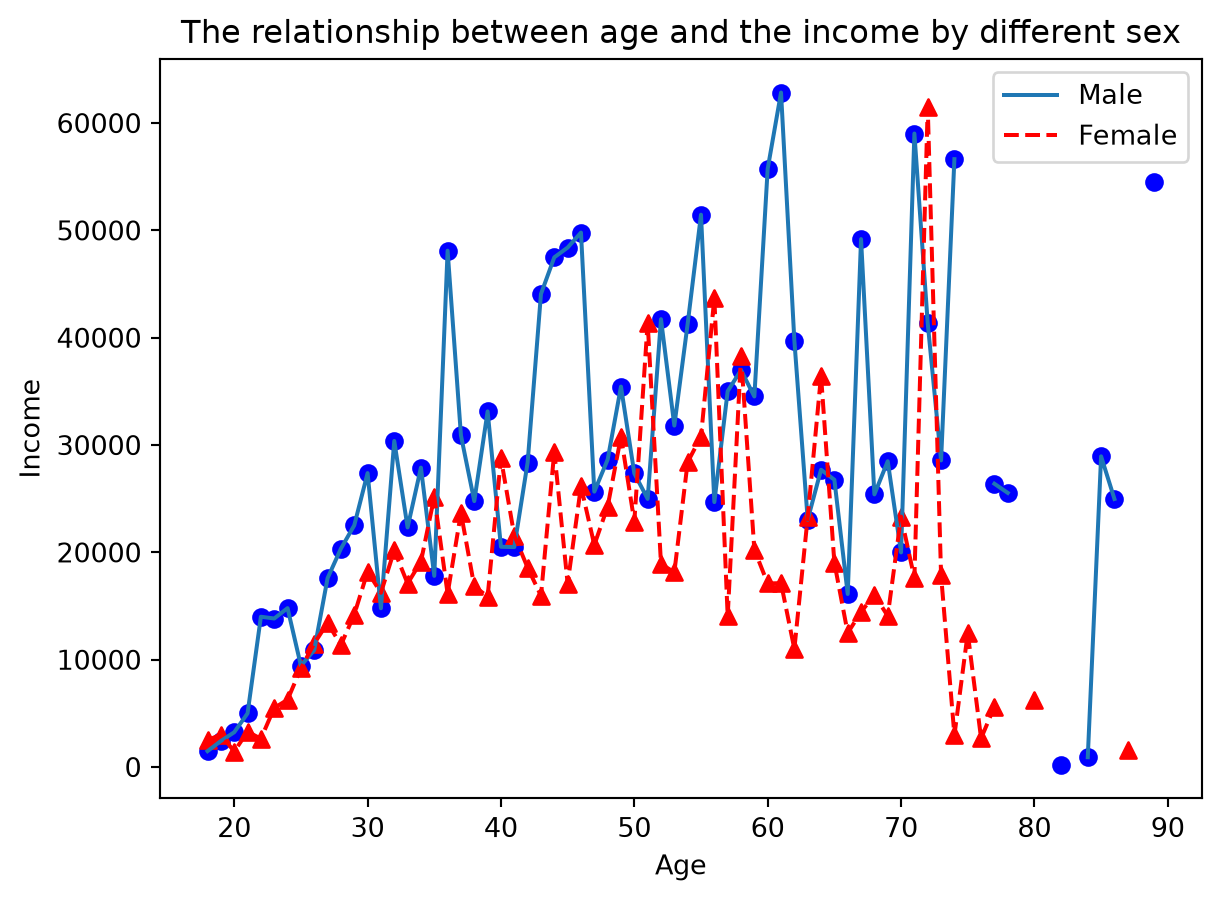
plt.plot(income_by_age_male['age'], income_by_age_male['realrinc'], label = 'Male')
# add title
plt.title('The relationship between age and the income by different sex')
# add x and y axis labels
plt.xlabel('Age')
plt.ylabel('Income')
# add points
plt.scatter(income_by_age_male['age'], income_by_age_male['realrinc'], color = 'blue')
# add a new line for sphrs1 using dotted line
plt.plot(income_by_age_female['age'], income_by_age_female['realrinc'], color = 'red', linestyle = '--', label = 'Female')
# add points for sphrs1 using a different triangle marker
plt.scatter(income_by_age_female['age'], income_by_age_female['realrinc'], color = 'red', marker = '^')
# add legend by color
plt.legend()
plt.show()

Saving and exporting

If you wish to export the data as a .csv file, you can use df.to_csv (export_file_path, index = False, header=True) to save your data set.

my_data.to_csv('exportmydata.csv', index = False, header=True)

Advanced Topics and Examples

While Python can handle most common statistical analyses, it is first and foremost a general purpose programming language. To truly leverage the unique advantages and flexibility of Python, knowledge of some additional programming concepts is necessary.

Control Flow - Loops

We often need to execute a set of commands/operations repeatedly. Instead of writing out the same set of code multiple times, we can encapsulate the piece of code within a looping code block.

There are 2 types of loops in Python.

The for loop is used when the number of iterations is predetermined and fixed before the looping block is executed. The loop ends when the last iteration is completed.

The while loop is used when the number of iterations is not predetermined. The loop ends when a specific condition is met. Hence, the number of iterations is not fixed.

a_num = [2,4,6,2,8,2,6,7,3,1]

for i in a_num:
  print(i)

for i in range(10):
  print(i)

c = 0
while c<len(a_num):
  print(a_num[c])
  c+=1


# Sometimes it may be necessary to enter the loop at least once and check the
# exit condition at the very end instead of the beginning
c = 0
while True:
  print(a_num[c])
  c+=1
  if c>=len(a_num): break

Functions

Functions are a set of well-defined and self-contained instructions that accomplishes a particular task. These are smaller modules of code that can be invoked from anywhere within the rest of programming code. Any Python command that is followed by () is a function.

Python functions start with the keyword def which means you are defining your own functions.

Next, it is followed by the function name and a set of parentheses, within which the function inputs are specified. After the inputs are specified, you go in to the function body. Note that the indentation always matters and your function body cannot be aligned with the keyword def. At the end of your function, if you need your function to return some outputs, you also need to specify what you want it to return. Functions in Python usually look something like this:

def FunctionName(input1, input2, input3):
    
    FunctionConditions
    
    return output

Now let’s look at an example of recoding the age variable into three categories, Young, Middle Aged, and Elder. To create this new variable, we only need to know the original numeric age values.

Now, we create our own function called transform_age which takes the numeric value of age as the function input. Within this function, the function body is a series of conditional statements of our coding schema. Since the recode variable is a string variable, we ask this transform_age function to return the corresponding categories.

Once we have this function, we can use the apply command to apply this function to the age variable and get what we want. We can use the unique() command to check that our transformation is indeed what we hoped for.

# When we have more than 2 categories (e.g., age)
# We will need to write a function to implement

def recode_age(age):
    if age > 75:
        return 'Elder'
    elif age >45:
        return 'Middle Aged'
    else:
        return 'Young'

# Check if function works
print(recode_age(80))
print(recode_age(50))

# Add a new column for the new categories
my_data['age_cat'] = my_data['age'].apply(recode_age)
my_data['age_cat']

# get the unique values in the column
my_data['age_cat'].unique()

# Count frequencies
my_data['age_cat'].value_counts()

Examples

The topics covered across Python I and Python II cover most of the fundamental concepts, commands, and data structures that underlie every Python module, library, or program.

Let’s look at an example of how we can combine all of these concepts to accomplish more complex tasks.

Scraping Wikipedia pages and generating wordclouds

# Load necessary libraries
# Corresponding documentation websites provided
import requests # https://requests.readthedocs.io/en/latest/
from bs4 import BeautifulSoup as bs # https://beautiful-soup-4.readthedocs.io/en/latest/
from wordcloud import WordCloud, STOPWORDS # https://amueller.github.io/word_cloud/index.html
import matplotlib.pyplot as plt # https://matplotlib.org/stable/index.html
from nltk.corpus import stopwords
import nltk # https://www.nltk.org/
import re # https://docs.python.org/3/library/re.html
import pandas as pd # https://pandas.pydata.org/docs/

# Download NLTK stopwords
nltk.download('stopwords')

# Function to get text from a Wikipedia page

def get_wiki_text(url):
    # Websites often require headers like user agent, cookies etc. to mask automated crawling activity.
    # Use this Google search query to find your current browser agent string https://www.google.com/search?q=my+browser+user+agent
    # There are more parameters that can be included in the header https://requests.readthedocs.io/en/latest/user/advanced/
    header = {'User-Agent':'Mozilla/5.0 (Windows NT 10.0; Win64; x64; rv:143.0) Gecko/20100101 Firefox/143.0'}

    response = requests.get(url, headers=header) # Sending an automated request and storing the data
    soup = bs(response.text, 'html.parser') # Parsing the response systematically
    paragraphs = soup.find_all('p') # Storing only text content
    text = ' '.join([p.text for p in paragraphs]) # Combining all paragraphs into a single document
    return text

languages = [
    'Python_(programming_language)',
    'R_(programming_language)',
    'JavaScript',
    'Java_(programming_language)'
]

# Dictionaries for storing text and wordcounts for each language as key:value pairs
language_word_counts = {}
language_texts = {}

for language in languages:
    # Create the Wikipedia URL
    url = f'https://en.wikipedia.org/wiki/{language}'

    # Get the text content
    text = get_wiki_text(url)
    language_texts[language] = text

    # Clean text - remove numbers and special characters
    cleaned_text = re.sub(r'[^a-zA-Z\s]', '', text)

    # Count unique words that are at least 3-letters long
    words = cleaned_text.lower().split()
    words = list(set(words))
    word_count = 0
    for word in words:
        if len(word) > 3 and word not in stopwords.words('english'):
            word_count += 1

    # Store the word count
    language_word_counts[language] = word_count
    print(f"{language.replace('_(programming_language)', '')}: {word_count} words")

# Function to generate and display wordcloud
def generate_wordcloud(text, title):
    combined_stopwords = STOPWORDS.union(set(stopwords.words('english')))
    wordcloud = WordCloud(
        stopwords=combined_stopwords,
        background_color='white',
        max_words=100,
        width=800,
        height=400
    ).generate(text)

    plt.figure(figsize=(10, 5))
    plt.imshow(wordcloud, interpolation='bilinear')
    plt.axis('off')
    plt.title(title)
    plt.show()

# Generate word clouds for each language
for language, text in language_texts.items():
    display_name = language.replace('_(programming_language)', '')
    generate_wordcloud(text, f"Word Cloud for {display_name}")

from scipy.stats import chi2_contingency

# Create a simple contingency table for two words - programming and object
words_to_check = ["programming", "object"]
contingency_table = []

for language in languages:
    # Clean text and convert to lowercase
    cleaned_text = re.sub(r'[^a-zA-Z\s]', '', language_texts[language]).lower()

    # Count occurrences of each word
    programming_count = cleaned_text.count(" programming ")
    object_count = cleaned_text.count(" object ")

    # Add to contingency table
    contingency_table.append([programming_count, object_count])

# Create a readable DataFrame for display
language_names = [lang.replace('_(programming_language)', '') for lang in languages]
contingency_df = pd.DataFrame(contingency_table,
                             index=language_names,
                             columns=words_to_check)

print("Contingency Table:")
print(contingency_df)

# Perform chi-square test using scipy library
chi2, p, dof, expected = chi2_contingency(contingency_table)

print("\nChi-square Independence Test Results:")
print(f"Chi-square statistic: {chi2:.4f}")
print(f"p-value: {p:.4f}")
print(f"Degrees of freedom: {dof}")
print(f"Interpretation: {'Word usage differs significantly across languages' if p < 0.05 else 'No significant difference in word usage across languages'}")

Common external libraries and frameworks across various domains

A non-comprehensive list of useful Python libraries with documentation links for further exploration.

Data Analysis & Statistics

pandas: Data manipulation and analysis
NumPy: Numerical computing with arrays and matrices
SciPy: Scientific computing (statistics, optimization, signal processing)
statsmodels: Statistical models and hypothesis testing
pingouin: Statistical analyses with simple API
pyMC: Bayesian statistical modeling and probabilistic machine learning

Data Visualization

Matplotlib: Basic plotting library
Seaborn: Statistical data visualization based on matplotlib
Plotly: Interactive visualizations
Folium: Interactive maps

Machine Learning & AI

scikit-learn: Classical machine learning algorithms
TensorFlow: Deep learning framework by Google
PyTorch: Deep learning framework by Facebook/Meta
Keras: High-level neural networks API
XGBoost: Gradient boosting implementation
Hugging Face Transformers: State-of-the-art NLP models

Natural Language Processing

NLTK: Natural Language Toolkit for text processing
spaCy: Industrial-strength NLP
gensim: Topic modeling and document similarity
TextBlob: Simplified text processing

Web Scraping & APIs

Requests: HTTP library for API calls
Beautiful Soup: HTML/XML parsing library
Scrapy: Web scraping framework
Selenium: Browser automation

Physical Sciences & Engineering

Astropy: Astronomy and astrophysics
Biopython: Biological computation
MDAnalysis: Molecular dynamics analysis
PyMOL: Molecular visualization
RDKit: Cheminformatics and computational chemistry
PyCaret: Low-code machine learning for scientific data
scikit-image: Image processing for scientific data

Bioinformatics & Genomics

Biopython: Processing biological data
scikit-bio: Bioinformatics algorithms
Pysam: Reading/writing genomic data formats
Bioconductor: (via rpy2) Genomic data analysis

Finance & Economics

pandas-datareader: Access to financial data
pyfolio: Portfolio and risk analytics
TA-Lib: Technical analysis library
Zipline: Algorithmic trading
arch: ARCH models for financial time series
statsmodels: Time series analysis
scikit-learn: Predictive modeling for financial data

Geospatial Analysis

GeoPandas: Geographic data handling
Rasterio: Raster data access
Shapely: Manipulation of geometric objects
PySAL: Spatial data science
Cartopy: Cartographic tools

Deep Learning Applications

OpenCV (cv2): Computer vision
librosa: Audio analysis
Transformers: NLP models
fastai: Vision, text, tabular data
Detectron2: Object detection
Kornia: Computer vision

Web Development

Django: Full-featured web framework
Flask: Lightweight web framework
Streamlit: Data apps with minimal code
Dash: Interactive analytic web applications
Gradio: Create UIs for machine learning models

Other Useful Libraries

tqdm: Progress bars for loops
pytest: Testing framework
Dask: Parallel computing
Ray: Distributed computing
SQLAlchemy: SQL toolkit and ORM
Pillow: Image processing
PyQt/PySide: GUI development
pygame: Game development

Introduction

Setup

Working With DataFrames: Data transformation

Creating a new variable

Recoding variables

Exercise 1

Inferential Statistics

Contingency table and chi-square test

Exercise 2

Independent samples t-test

Exercise 3

ANOVA

Exercise 4

Correlation Matrix

Linear Regression

Visualizations

Histogram

Bar graphs

Exercise 5

Scatterplot

Using Matplotlib library for advanced visualizations

Scatterplot

Line chart

Multiple charts

Saving and exporting

Advanced Topics and Examples

Control Flow - Loops

Functions

Examples

Scraping Wikipedia pages and generating wordclouds

Common external libraries and frameworks across various domains

Data Analysis & Statistics

Data Visualization

Machine Learning & AI

Natural Language Processing

Web Scraping & APIs

Social Sciences

Physical Sciences & Engineering

Bioinformatics & Genomics

Finance & Economics

Geospatial Analysis

Deep Learning Applications

Web Development

Other Useful Libraries